A literate Lattice Boltzmann Code

Adrian Kummerländer

What?

Literate Programming

…a tool for reproducible science.

Instead of imagining that our main task is to instruct a computer what to do, let us concentrate rather on explaining to human beings what we want a computer to do. —Donald Knuth (Literate Programming, 1984)

Setup

Emacs text edtor with org-babel
Literate source file can be …
… tangled to a compilable program
… woven into a prose document (e.g. HTML / PDF)
Languages may be easily mixed

LiterateLB Features

Self contained
(Smagorinsky) BGK collision
Workable set of boundary conditions
Integrated (volumetric) visualization
Interesting set of examples
Competitive GPU performance

Visualization

Useful both for science and art
Just in Time vs. Real Time
Inspired by reality and freed from its restrictions

Signed Distance Functions

\(d : \mathbb{R}^3 \to \mathbb{R}\) is shortest distance to surface
Iteratively approximate directed distances
Surface normals
Model for boundary configuration and visualization

Constructive Solid Geometry

library of geometric primitives
combine with boolean operators

v = translate(v, center);

return ssub(
    rounded(box(v, v3(20, 20, 20)), 5),
    sphere(v, 25),
    5
);

Fancy example

add(
  sadd(
    sub(
      rounded(box(v, v3(5, 28, 38)), 1),
      rounded(box(v, v3(6, 26, 36)), 1)
    ),
    cylinder(translate(v, v3(0,0,-45)), 5, 12),
    1
  ),
  sintersect(
    box(v, v3(5, 28, 38)),
    add(
      add(
        box(rotate_x(v, angle), v3(10, width, 100)),
        box(rotate_x(v, -angle), v3(10, width, 100))
      ),
      add(
        add(
          add(
            box(rotate_x(translate(v, v3(0,0,25)), angle), v3(10, width, 100)),
            box(rotate_x(translate(v, v3(0,0,25)), -angle), v3(10, width, 100))
          ),
          add(
            box(rotate_x(translate(v, v3(0,0,-25)), angle), v3(10, width, 100)),
            box(rotate_x(translate(v, v3(0,0,-25)), -angle), v3(10, width, 100))
          )
        ),
        add(
          add(
            box(rotate_x(translate(v, v3(0,0,50)), angle), v3(10, width, 100)),
            box(rotate_x(translate(v, v3(0,0,50)), -angle), v3(10, width, 100))
          ),
          add(
            box(rotate_x(translate(v, v3(0,0,-50)), angle), v3(10, width, 100)),
            box(rotate_x(translate(v, v3(0,0,-50)), -angle), v3(10, width, 100))
          )
        )
      )
    ),
    2
  )
);

Sphere tracing

Volumetric Visualization

Ray Marching

Common practice for volume rendering
Periodically sample some scalar value along a ray
… velocity norm, density, curl magnitude, shear layer visibility, various quality criteria …
Discretized volume rendering equation
Extensible to arbitrarily complex light transport

Volume rendering equation

Color \(C\) along ray \(r\) with length \(L\) with absorption \(\mu\): \[C(r) = \int_0^L c(x) \mu(x) \exp\left(-\int_0^x \mu(t) dt\right) dx\]

Simplified for speed: \[C(r) = \sum_{i=0}^N C(i \Delta x) \alpha (i \Delta x) \prod_{j=0}^{i-1} \left(1 - \alpha(j\Delta x)\right)\]

Color palette

Can make or break a good visualization
SciVisColor.org offers a variety of useful palettes
LiterateLB includes a selection of them

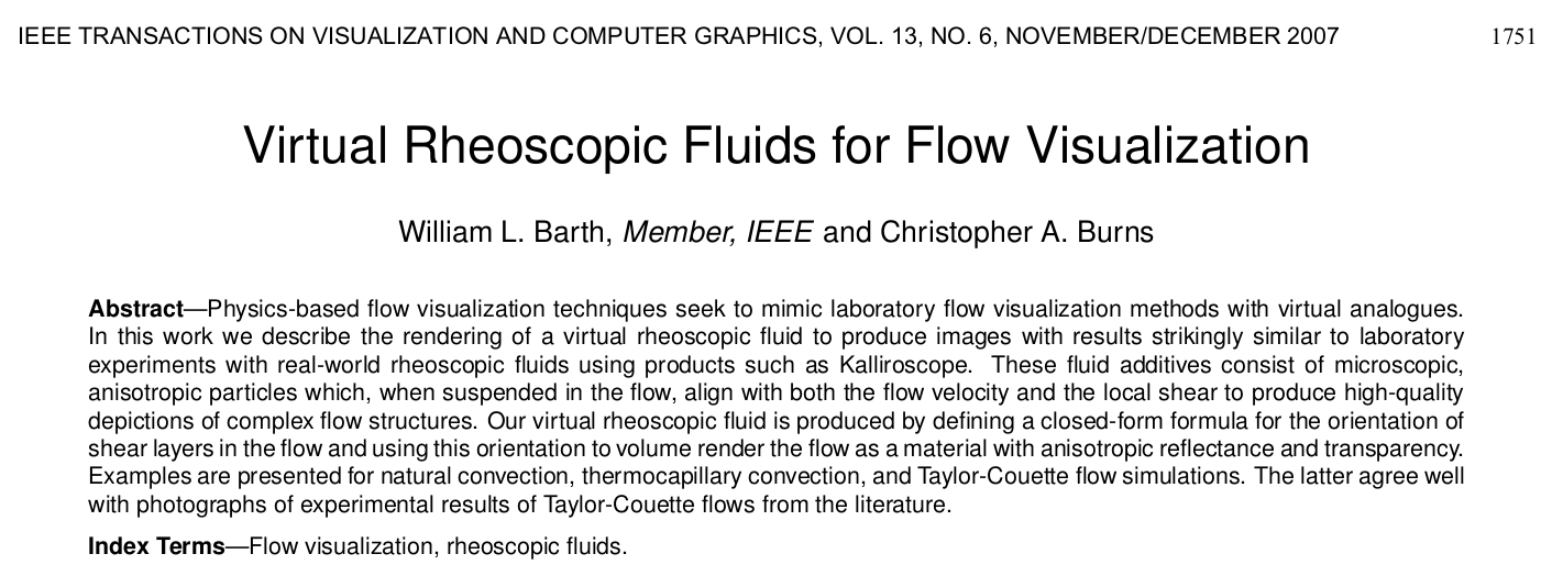
Virtual Rheoscopic Fluid

\(n_\text{shear} = 2 D u \hat{u} - 2\left(u^T D u \hat{u} \right) \hat{u}\)

Shear Layer Normal

fuid stress tensor \(\sigma\), strain-rate tensor \(Du\)
\(R_{\hat{u}} = \sigma \hat{u}\) force on infinitesimal plane in flow
\(R_{\hat{u}} - (R_{\hat{u}} \cdot \hat{u}) \hat{u} = 2\mu Du\hat{u} - 2\mu(\hat{u}^TDu\hat{u})\hat{u}\)
Neglect viscosity scalar \[n_\text{shear} = 2 D u \hat{u} - 2\left(u^T D u \hat{u} \right) \hat{u}\]
Construct strain-rate tensor from \(f^\text{neq}\)