A literate Lattice Boltzmann Code

Adrian Kummerländer

This file describes a full Lattice Boltzmann code featuring both 2D and 3D lattices, a workable selection of boundary conditions, Smagorinsky turbulence modelling, expression-level code optimization and even a full ray marcher for just-in-time volumetric visualization in addition to a set of interesting examples. All of this runs on GPUs using CUDA near the maximum possible performance on that platform.

This document is a work in progress.

1. Introduction

Approaches to modeling fluid dynamics can be coarsely grouped into three categories: Microscopic, Mesoscopic and Macroscopic models. Microscopic models describe the behavior of the individual particles of whose the macroscopic fluid movement is an emergent property. On the other side of the spectrum, macroscopic models consider only the large scale properties of a fluid such as its velocity and density fields. One could say that microscopic particle models are closest to what actually happens in nature and macroscopic models in the form of the Navier Stokes equations (NSE) represent an ideal vision of a fluid that only holds for large enough space scales. As is the case for most things, what we call a fluid is by itself already an abstraction.

Mesoscopic models sit between these two extremes and consider neither individual particles nor purely macroscopic properties but rather the probability of some amount of particles moving with some velocity into a certain direction at various points in time and space. The mathematical field of kinetic theory provides a foundation for linking all of these three models.

1.1. Kinetic Theory

One can use kinetic theory to get from a microscropic or molecular system governed by e.g. Newton's laws of motion to macroscopic descriptions of certain properties of such a system. For example one can reach the diffusion equation for billiard systems of particles colliding with solid obstacles or to the Navier Stokes equations for systems of pairwise colliding particles.

In very rough terms one starts out by considering the microscopic system and taking its limit for infinitely many particles of vanishingly small size. This yields a kinetic equation that describes the behaviour of the particle distribution function under some collision operator for any point in space and time. When we consider pairwise colliding particles the result turns out to be the well known Boltzmann transport equation:

\[(\partial_t + v \cdot \nabla_x) f(t,x,v) = \Omega (f).\]

This PDE describes the behavior of the probability \(f(t,x,v)\) that particles move into direction \(v\) at location \(x\) and time \(t\) for some collision operator \(\Omega\). Discretizing this equation on a lattice for a finite set of discrete velocities is called the Lattice Boltzmann Method (LBM).

The practical usefulness of LBM hinges on the ability of reaching the desired target equations such as NSE or the heat equation as a limit of the kinetic equation.

1.2. Lattice Boltzmann Method

We discretize the Boltzmann equation in spatial, velocity and temporal space on a cartesian lattice using discrete velocities \(\xi_i\) that point to the neighbors of each cell.

\[(\partial_t + v \cdot \nabla_x)f = \Omega(f) \approx f_i(x + \xi_i, t + 1) - f_i(x,t) = \Omega_i(x,t)\]

A common collision operator \(\Omega\) for Navier-Stokes approximation is given by Bhatnagar, Gross and Kroog (BGK).

\[\Omega(f) := -\frac{f - f^\text{eq}}{\tau}\]

This BGK operator relaxes the local population \(f\) towards some equilibrium distribution \(f^\text{eq}\) with rate \(\tau\). Inserting this operator into the discrete Boltzmann equation yields the discrete LBM BGK equation.

\[f_i(x + \xi_i, t + 1) = f_i(x,t) - \frac{1}{\tau} (f_i(x,t) - f_i^\text{eq}(x,t))\]

This explicit form exposes the separation of the LBM algorithm into a local collision step followed by a streaming step. The collision step relaxes the population of each cell towards its local equilibrium and the streaming step propagates the resulting updated population values to the respective neighboring cells.

Macroscopic moments such as density and velocity can be calculated directly from the distribution functions.

\[\rho := \sum_{i=0}^{q-1} f_i(x,t) \text{ and } u := \frac{1}{\rho} \sum_{i=0}^{q-1} \xi_i f_i(x,t)\]

The equilibrium distribution \(f_i^\text{eq}\) for these macroscopic properties is given by

\[f_i^\text{eq}(x,t) := \omega_i \rho \left( 1 + \frac{u \cdot \xi_i}{c_s^2} + \frac{(u \cdot \xi_i)^2}{2c_s^4} - \frac{u \cdot u}{2c_s^2} \right)\]

using lattice-dependent weights \(\omega_i\) and speed of sound \(c_s\). Note that this is just one possible discretization of the Boltzmann equation – nothing stops us from using different sets of velocities, relaxation times, collision operators and so on. Changing these things is how different physics are modeled in LBM. e.g. what we will do in the section on Smagorinsky turbulence modelling is to locally change the relaxation time.

To summarize what we are going to do for the simplest bulk fluid case: First calculate the current density and velocity moments of a cell, then compute the matching equilibrium distributions and finally perform the local BGK collision to update the cell populations. The last step before we start again is to propagate the post-collision values to the corresponding neighbor cells.

Special care has to be taken for the boundary conditions at the lattice frontier and around any obstacle geometries. Such boundary conditions are one of the major topics of LBM research with a very rich toolbox of specialized collision steps for modeling e.g. inflow, outflow, solid or moving walls of various kinds.

As a starting point for further reading on LBM I can recommend the de facto standard text [3] by Krüger et al.

1.3. Literate Programming

The present website is the documentation woven from the literate program file lbm.org. In the same fashion this program file may also be tangled into compilable code. Programs written using this paradigm are commonly referred to as literate and promise to decouple program exposition from the strict confines of machine-targeted languages.

LiterateLB utilizes the literate programming framework offered by Emacs's Org Mode.

The easiest way to tangle and compile the project is to use the Nix package manager. On CUDA-enabled NixOS hosts the following commands are all that is needed to tangle, compile and run one of the simulation examples:

git clone https://code.kummerlaender.eu/LiterateLB
cd LiterateLB
nix build
./result/bin/nozzle

On other systems the dependencies

Emacs 28 (earlier possible for up-to-date orgmode)
CMake 3.10 or later
Nvidia CUDA 10.2 or later
SFML 2.5 or later and ImGui-SFML
Python with SymPy, NumPy, SciPy and Mako

will have to be provided manually. Note that the current tangle output is included so strictly speaking compiling and testing the examples requires neither Emacs nor Python.

Note that I started developing this as a beginner in both Emacs and Org mode so some aspects of this document may be more clunky than necessary. Most of the complexity stems from maintaining a Python session for the generation of optimized GPU kernel functions using the SymPy CAS:

2. Lattice

The cartesian grids used for the spatial discretization are commonly described as DXQY lattices where X is the number of spatial dimensions and Y is the number of discrete velocities \(\xi_i\). e.g. a D2Q9 lattice is two dimensional and stores nine population values per cell. Each population has an associated weigth \(\omega_i\) that in a sense controls its impact on the collision step. Additionally we also require the lattice speed of sound \(c_s\) which is the speed of information propagation within the lattice.

from fractions import Fraction

class Descriptor:
    def __init__(self, name, data):
        self.name = name
        self.c = [ Matrix(eval(row[0]))    for row in data ]
        self.w = [ Rational(f.numerator, f.denominator)
                   for f in [ Fraction(row[1]) for row in data ] ]
        
        self.d = self.c[0].shape[0]
        self.q = len(self.c)
        self.c_s = sqrt(Rational(1,3))

All of these constants have to be accessible for symbolic computations which is why we store them within a so called descriptor class. For convenience we write out the directions and weights as plain tables that are then read into the Python structure.

descriptor[lattice] = Descriptor(lattice, data)
print(f"Loaded D{descriptor[lattice].d}Q{descriptor[lattice].q} lattice with a weight sum of {sum(descriptor[lattice].w)}.")

Loaded D2Q9 lattice with a weight sum of 1.

Loaded D3Q19 lattice with a weight sum of 1.

2.1. D2Q9

Direction	Weight
(-1,-1)	1/36
(-1, 0)	1/9
(-1, 1)	1/36
( 0,-1)	1/9
( 0, 0)	4/9
( 0, 1)	1/9
( 1,-1)	1/36
( 1, 0)	1/9
( 1, 1)	1/36

2.2. D3Q19

Direction	Weight
( 0, 1, 1)	1/36
(-1, 0, 1)	1/36
( 0, 0, 1)	1/18
( 1, 0, 1)	1/36
( 0,-1, 1)	1/36
(-1, 1, 0)	1/36
( 0, 1, 0)	1/18
( 1, 1, 0)	1/36
(-1, 0, 0)	1/18
( 0, 0, 0)	1/3
( 1, 0, 0)	1/18
(-1,-1, 0)	1/36
( 0,-1, 0)	1/18
( 1,-1, 0)	1/36
( 0, 1,-1)	1/36
(-1, 0,-1)	1/36
( 0, 0,-1)	1/18
( 1, 0,-1)	1/36
( 0,-1,-1)	1/36

3. Collision Steps

While the streaming step of the LBM algorithm only propagates the populations between cells in an unform fashion, the collision step determines the actual values those populations take. This means that the physical behaviour modelled by a given LBM algorithm is determined primarily by the collision step.

In this section we are going to generate the code for bulk collisions. i.e. the collisions that model fluid and other transport phenomena apart from domain boundaries. Those will be handled at a later point by special purpose collision steps called boundary conditions.

3.1. Code printing

Before we can get started on constructing expression trees and generating code from them we need to setup some basics so SymPy actually generates something we can compile in our environment.

In order to get more fine grained control we need to overload an approproate SymPy C code printer class. This allows us to e.g. easily print indexed expressions that access the population array in the correct way or to explicitly type float constants according to a compile-time template type.

from sympy.printing.ccode import C11CodePrinter

class CodeBlockPrinter(C11CodePrinter):
    def __init__(self, custom_assignment, custom_functions):
        super(CodeBlockPrinter, self).__init__()
        self._default_settings['contract'] = False
        self.custom_assignment = custom_assignment
        for f in custom_functions:
            self._kf[f] = f
    
    def _print_Indexed(self, expr):
        assert len(expr.indices) == 1
        if expr.base.name[0] == 'f':
            return f"{expr.base.name}[{expr.indices[0]}]"
        else:
            return f"{expr.base.name}_{expr.indices[0]}"
    
    def _print_Float(self, flt):
        return "T{%s}" % str(flt.evalf())

    def _print_Pow(self, expr):
        if expr.exp == -1:
            return "T{1} / (%s)" % self.doprint(expr.base)
        else:
            return super()._print_Pow(expr)

    def _print_Assignment(self, expr):
        if self.custom_assignment and expr.lhs.is_Indexed and expr.lhs.base.name[0] == 'f':
            return f"{self.doprint(expr.lhs)} = {self.doprint(expr.rhs.evalf())};"
        else:
            return f"T {self.doprint(expr.lhs)} = {self.doprint(expr.rhs.evalf())};"

For convenience the instantiation of this class is hidden in a printcode function that we can use everywhere.

def printcode(expr, custom_assignment=True, custom_functions=[]):
    print(CodeBlockPrinter(custom_assignment, custom_functions).doprint(expr))

The additional assignment parameter allow us to control whether the targets of assignment expressions should be instantiated as a new scalar variable in addition while the functions parameter allows us to make custom runtime functions known to SymPy. If we don't do this for a function f that our assignment expression contains a reference to, the printer will generate unwanted comments to reflect this.

3.1.1. Custom expression transformations

We do not want to use the pow function for squares in the generated code. This can be achieved by providing a custom ReplaceOptim structure during the CSE optimization step that conditionally resolves Pow expressions.

from sympy.codegen.rewriting import ReplaceOptim
from sympy.simplify import cse_main

expand_pos_square = ReplaceOptim(
    lambda e: e.is_Pow and e.exp.is_integer and e.exp == 2,
    lambda p: UnevaluatedExpr(Mul(p.base, p.base, evaluate = False))
)

custom_opti = cse_main.basic_optimizations + [
    (expand_pos_square, expand_pos_square)
]

def cse(block, symbol_prefix = 'x'):
    return block.cse(symbols = numbered_symbols(prefix=symbol_prefix), optimizations = custom_opti, order = 'none')

3.2. Moments

i, j = symbols('i, j')
d, q = symbols('d, q')
xi = IndexedBase('xi')

To start we define placeholders for the spatial and discrete velocity dimensions as well as the velocity set \(\xi\) of some lattice. As the moments are constructed using the lattice populations \(f\) we also require placeholders for those in addition to the moments \(\rho\) and \(u\) themselves.

f = IndexedBase('f')
rho = Symbol('rho')
u = IndexedBase('u', d)
u_i = Symbol('u_i')

We are now ready to formulate the density moment which is simply the sum of a cell's populations.

def rho_from_f(f, q):
    return Assignment(rho, Sum(f[j], (j, 0, q-1)))

printlatexpr(rho_from_f(f, q))

\[\begin{align*} \rho &:= \sum_{j=0}^{q - 1} {f}_{j} \\ \end{align*}\]

Next we build the velocity moment function. The i-th component of the velocty \(u\) is the sum of all relevant populations divided by the density. In this context relevant populations are all values \(f_j\) for which the i-th component of velocity \(\xi_j\) is non-zero.

def u_i_from_f(f, q, xi):
    return Assignment(u_i, Sum(xi[j,i] * f[j], (j, 0, q-1)) / Sum(f[j], (j, 0, q-1)))

printlatexpr(u_i_from_f(f, q, xi))

\[\begin{align*} u_{i} &:= \frac{\sum_{j=0}^{q - 1} {f}_{j} {\xi}_{j,i}}{\sum_{j=0}^{q - 1} {f}_{j}} \\ \end{align*}\]

Both to illustrate what we are actually going to compute for a given lattice cell and as the next step towards code generation we now want to realize our abstract moment expressions for a concrete lattice.

def realize_rho(D):
    return rho_from_f(f, D.q).doit()

D = descriptor[lattice]
printlatexpr(realize_rho(D))

\[\begin{align*} \rho &:= {f}_{0} + {f}_{1} + {f}_{2} + {f}_{3} + {f}_{4} + {f}_{5} + {f}_{6} + {f}_{7} + {f}_{8} \\ \end{align*}\]

def from_indices(elems, car, *cdr):
    return elems[car] if len(cdr) == 0 else from_indices(elems[car], *cdr)

def realize_indexed(expr, idx, values):
    return expr.replace(lambda expr: expr.is_Indexed and expr.base.name == idx.name,
                        lambda elem: from_indices(values, *elem.indices))

def realize_u_i(D, j):
    return realize_indexed(u_i_from_f(f, D.q, xi).doit().subs([(u_i, u[j]), (i, j)]), xi, D.c)

D = descriptor[lattice]
printlatexpr(realize_u_i(D, 0))

\[\begin{align*} {u}_{0} &:= \frac{- {f}_{0} - {f}_{1} - {f}_{2} + {f}_{6} + {f}_{7} + {f}_{8}}{{f}_{0} + {f}_{1} + {f}_{2} + {f}_{3} + {f}_{4} + {f}_{5} + {f}_{6} + {f}_{7} + {f}_{8}} \\ \end{align*}\]

At this point we have everything needed to generate an optimized code snippet that can be used to compute density and velocity values given a set of variables containing a single cell's populations. As a convention we are going to prefix these current population variables with f_curr.

def moments_code_block(D, populations):
    f_rho = realize_indexed(realize_rho(D), f, populations)
    f_u = [ realize_indexed(realize_u_i(D, i), f, populations) for i in range(D.d) ]
    return CodeBlock(f_rho, *f_u).cse(symbols = numbered_symbols(prefix='m'), optimizations = custom_opti)

printcode(moments_code_block(descriptor[lattice], IndexedBase('f_curr')))

T m0 = f_curr[1] + f_curr[2];
T m1 = f_curr[3] + f_curr[6];
T m2 = m0 + m1 + f_curr[0] + f_curr[4] + f_curr[5] + f_curr[7] + f_curr[8];
T m3 = f_curr[0] - f_curr[8];
T m4 = T{1} / (m2);
T rho = m2;
T u_0 = -m4*(m0 + m3 - f_curr[6] - f_curr[7]);
T u_1 = -m4*(m1 + m3 - f_curr[2] - f_curr[5]);

Both the fluid dynamics implemented by collision steps and boundary conditions as well as functions for computing moments to e.g. visualize are implemented as GPU kernel functions. In CUDA this means plain functions marked by the __global__ specifier. As most kernel share common aspects in their call requirements and parameter sets we wrap them in __device__ functions of sensibly named structures.

#pragma once
#include <LLBM/call_tag.h>

struct CollectMomentsF {

using call_tag = tag::call_by_cell_id;

template <typename T, typename S>
__device__ static void apply(descriptor::D2Q9, S f_curr[9], std::size_t gid, T* cell_rho, T* cell_u) {
  <<moments-from-f_curr(lattice="D2Q9")>>

  cell_rho[gid] = rho;
  cell_u[2*gid+0] = u_0;
  cell_u[2*gid+1] = u_1;
}

template <typename T, typename S>
__device__ static void apply(descriptor::D3Q19, S f_curr[19], std::size_t gid, T* cell_rho, T* cell_u) {
  <<moments-from-f_curr(lattice="D3Q19")>>

  cell_rho[gid] = rho;
  cell_u[3*gid+0] = u_0;
  cell_u[3*gid+1] = u_1;
  cell_u[3*gid+2] = u_2;
}

};

3.3. Equilibrium

f_eq = IndexedBase('f_eq', q)

\[f_i^\text{eq}(x,t) := \omega_i \rho \left( 1 + \frac{u \cdot \xi_i}{c_s^2} + \frac{(u \cdot \xi_i)^2}{2c_s^4} - \frac{u \cdot u}{2c_s^2} \right)\]

Calculating the equilibrium distribution of some population \(f_i\) requires the evaluation of inner products between vectors. As there doesn't seem to be a nice way of writing an abstract SymPy expression that both generates nice LaTeX and can be realized on a concrete lattice we skip the fully abstract step and jump right into the latter part.

def realize_f_eq_i(D, i):
    v = Matrix([ u[j] for j in range(D.d) ])
    return Assignment(f_eq[i], D.w[i] * rho * ( 1
                                              + D.c[i].dot(v)    /    D.c_s**2
                                              + D.c[i].dot(v)**2 / (2*D.c_s**4)
                                              - v.dot(v)         / (2*D.c_s**2) ))

D = descriptor[lattice]
printlatexpr(realize_f_eq_i(D, 0))

\[\begin{align*} {f_{eq}}_{0} &:= \frac{\rho \left(\frac{9 \left(- {u}_{0} - {u}_{1}\right)^{2}}{2} - \frac{3 {u}_{0}^{2}}{2} - 3 {u}_{0} - \frac{3 {u}_{1}^{2}}{2} - 3 {u}_{1} + 1\right)}{36} \\ \end{align*}\]

def equilibrium_code_block(D):
    f_moment_eq = [ Assignment(f_next[i], realize_f_eq_i(D, i).rhs) for i in range(D.q) ]
    return cse(CodeBlock(*f_moment_eq), symbol_prefix = 'e')

printcode(equilibrium_code_block(descriptor[lattice]))

T e0 = T{0.0277777777777778}*rho;
T e1 = T{3.00000000000000}*u_1;
T e2 = T{3.00000000000000}*u_0;
T e3 = u_0 + u_1;
T e4 = T{4.50000000000000}*(e3*e3);
T e5 = u_1*u_1;
T e6 = T{1.50000000000000}*e5;
T e7 = u_0*u_0;
T e8 = T{1.50000000000000}*e7;
T e9 = e8 + T{-1.00000000000000};
T e10 = e6 + e9;
T e11 = T{0.111111111111111}*rho;
T e12 = -e2;
T e13 = T{1.00000000000000} - e6;
T e14 = e13 + T{3.00000000000000}*e7;
T e15 = -e8;
T e16 = e1 + e15;
T e17 = u_0 - u_1;
T e18 = e13 + T{4.50000000000000}*(e17*e17);
T e19 = T{3.00000000000000}*e5;
f_next[0] = -e0*(e1 + e10 + e2 - e4);
f_next[1] = e11*(e12 + e14);
f_next[2] = e0*(e12 + e16 + e18);
f_next[3] = -e11*(e1 - e19 + e9);
f_next[4] = -T{0.444444444444444}*e10*rho;
f_next[5] = e11*(e16 + e19 + T{1.00000000000000});
f_next[6] = e0*(-e1 + e15 + e18 + e2);
f_next[7] = e11*(e14 + e2);
f_next[8] = e0*(e13 + e16 + e2 + e4);

3.4. BGK Collision

The BGK collision operators takes a current population \(f^{curr}_i\) and relaxes it toward the equilibrium distribution \(f^{eq}_i\) with some rate \(\tau\). The result of this process is the new population \(f^{next}_i\).

tau = Symbol('tau')
f_curr = IndexedBase('f_curr', q)
f_next = IndexedBase('f_next', q)
f_curr_i, f_next_i, f_eq_i = symbols('f^curr_i, f^next_i, f^eq_i')

def bgk_collision(f_curr, f_next, f_eq, tau):
    return Assignment(f_next, f_curr + 1/tau * (f_eq - f_curr))

printlatexpr(bgk_collision(f_curr_i, f_next_i, f_eq_i, tau))

\[\begin{align*} f^{next}_{i} &:= f^{curr}_{i} + \frac{- f^{curr}_{i} + f^{eq}_{i}}{\tau} \\ \end{align*}\]

As we might want to use different moment values than the ones constructed from the current population as the foundation for the equilibrium distribution the generated code will assume variables rho and u_i to exist. Building the expression tree for code generation is now as simple as instantiating the BGK operator for all \(q\) directions and substituting the equilibrium distribution.

def bgk_collision_code_block(D):
    f_eq_def = [ realize_f_eq_i(D, i).rhs for i in range(D.q) ]
    f_post_collide = [ bgk_collision(f_curr[i], f_next[i], f_eq_def[i], tau) for i in range(D.q) ]
    return CodeBlock(*f_post_collide).cse(optimizations = custom_opti)

printcode(bgk_collision_code_block(descriptor[lattice]), custom_assignment=True)

T x0 = T{1} / (tau);
T x1 = T{0.0138888888888889}*x0;
T x2 = T{6.00000000000000}*u_1;
T x3 = T{6.00000000000000}*u_0;
T x4 = u_0 + u_1;
T x5 = T{9.00000000000000}*(x4*x4);
T x6 = u_1*u_1;
T x7 = T{3.00000000000000}*x6;
T x8 = u_0*u_0;
T x9 = T{3.00000000000000}*x8;
T x10 = x9 + T{-2.00000000000000};
T x11 = x10 + x7;
T x12 = T{0.0555555555555556}*x0;
T x13 = -x3;
T x14 = T{2.00000000000000} - x7;
T x15 = x14 + T{6.00000000000000}*x8;
T x16 = -x9;
T x17 = x16 + x2;
T x18 = u_0 - u_1;
T x19 = x14 + T{9.00000000000000}*(x18*x18);
T x20 = T{6.00000000000000}*x6;
f_next[0] = -x1*(rho*(x11 + x2 + x3 - x5) + T{72.0000000000000}*f_curr[0]) + f_curr[0];
f_next[1] = x12*(rho*(x13 + x15) - T{18.0000000000000}*f_curr[1]) + f_curr[1];
f_next[2] = x1*(rho*(x13 + x17 + x19) - T{72.0000000000000}*f_curr[2]) + f_curr[2];
f_next[3] = -x12*(rho*(x10 + x2 - x20) + T{18.0000000000000}*f_curr[3]) + f_curr[3];
f_next[4] = -T{0.111111111111111}*x0*(T{2.00000000000000}*rho*x11 + T{9.00000000000000}*f_curr[4]) + f_curr[4];
f_next[5] = x12*(rho*(x17 + x20 + T{2.00000000000000}) - T{18.0000000000000}*f_curr[5]) + f_curr[5];
f_next[6] = x1*(rho*(x16 + x19 - x2 + x3) - T{72.0000000000000}*f_curr[6]) + f_curr[6];
f_next[7] = x12*(rho*(x15 + x3) - T{18.0000000000000}*f_curr[7]) + f_curr[7];
f_next[8] = x1*(rho*(x14 + x17 + x3 + x5) - T{72.0000000000000}*f_curr[8]) + f_curr[8];

In order to call this collision kernel on the GPU we wrap it in apply functions of an appropriately named operator structure.

#pragma once
#include <LLBM/call_tag.h>

struct BgkCollideO {

using call_tag = tag::call_by_cell_id;

template <typename T, typename S>
__device__ static void apply(descriptor::D2Q9, S f_curr[9], S f_next[9], std::size_t gid, T tau) {
  <<moments-from-f_curr(lattice="D2Q9")>>
  <<bgk-collide-to-f_next(lattice="D2Q9")>>
}

template <typename T, typename S>
__device__ static void apply(descriptor::D3Q19, S f_curr[19], S f_next[19], std::size_t gid, T tau) {
  <<moments-from-f_curr(lattice="D3Q19")>>
  <<bgk-collide-to-f_next(lattice="D3Q19")>>
}

};

#include "kernel/collide.h"

3.5. Smagorinsky BGK Collision

Simulation of turbulent flow using plain BGK collisions is possible – after all turbulence is captured by the Navier-Stokes equations that in turn are the target equations of our BGK-LB method – but requires very highly resolved grids. The reason for this is that turbulence is characterized by the formation of eddies at both very big and very small scales. Most of the energy is contained in the large scale features but dissipates into heat at the finest scales. To capture turbulent flow we either have to resolve the grid all the way to these finest scales or implement some kind of model for the characteristics of these scales in a coarser grid. Computation on such a coarser grid is then also called a large eddy simulation (LES).

One comparably simple model for respresenting the smaller eddies in such a LES is the Smagorinsky subgrid-scale model. This model yields a expression for computing the effective relaxation rate \(\tau_\text{eff}\) on a per-cell basis given the global relaxation time \(\tau\) and a Smagorinsky constant. As the relaxation time in BGK LBM is a function of the viscosity this translates into computing the effective viscosity using a local strain-rate tensor reconstruction based on the non-equilibrium part of each cell's populations. This follows the approach laid out by Yu et al. in [1].

tau, smagorinsky = symbols('tau, smagorinsky')

The non-equilibrium part is simply the difference between the actual population stored in a cell and the respective equilibrium population that we relax towards. Using these local non-equilibrium parts to reconstruct the strain-rate tensor \(\Pi_{i,j}^\text{neq}\) is quite convenient as we otherwise would have to employ e.g. a finite difference method just for this.

def pi_neq(D, f, f_eq):
    pi_neq = zeros(D.d, D.d)
    for i, j, k in multirange(D.d, D.d, D.q):
        pi_neq[i,j] += D.c[k][i] * D.c[k][j] * (f[k] - f_eq[k])
    
    return pi_neq

To compute the effective relaxation rate we need the norm of this strain-rate tensor.

def pi_neq_norm(D, f, f_eq):
    pi = pi_neq(D, f, f_eq)
    return sqrt(2*multisum(lambda i, j: pi[i,j]**2, D.d, D.d))

def effective_tau(D, f, f_eq, tau, smagorinsky):
    pi_norm = pi_neq_norm(D, f, f_eq)
    return tau + 0.5*(sqrt(tau**2 + 2*sqrt(2)*smagorinsky**2 * pi_norm / D.c_s**4) - tau)

Finally the resulting per-cell relaxation time is simply plugged into the existing BGK collision operator to yield the complete Smagorinsky BGK collision step.

def smagorinsky_bgk_collision_code_block(D, tau, smagorinsky):
    f_rho = realize_indexed(realize_rho(D), f, f_curr)
    f_u = [ realize_indexed(realize_u_i(D, i), f, f_curr) for i in range(D.d) ]
    f_eq = [ realize_f_eq_i(D, i).rhs for i in range(D.q) ]
    eff_tau = effective_tau(D, f_curr, f_eq, tau, smagorinsky)
    f_post_collide = [ bgk_collision(f_curr[i], f_next[i], f_eq[i], eff_tau) for i in range(D.q) ]
    return CodeBlock(f_rho, *f_u, *f_post_collide).cse(optimizations = custom_opti)

This way the BGK collisions are numerically stabilized for low resolutions and high Reynolds numbers.

D = descriptor[lattice]
printcode(smagorinsky_bgk_collision_code_block(D, tau, smagorinsky))

T x0 = f_curr[1] + f_curr[2];
T x1 = f_curr[3] + f_curr[6];
T x2 = x0 + x1 + f_curr[0] + f_curr[4] + f_curr[5] + f_curr[7] + f_curr[8];
T x3 = f_curr[0] - f_curr[8];
T x4 = T{1} / (x2);
T x5 = T{72.0000000000000}*f_curr[2];
T x6 = T{72.0000000000000}*f_curr[6];
T rho = x2;
T x31 = T{4.00000000000000}*rho;
T x40 = T{2.00000000000000}*rho;
T u_0 = -x4*(x0 + x3 - f_curr[6] - f_curr[7]);
T x7 = T{6.00000000000000}*u_0;
T x8 = -x7;
T x15 = u_0*u_0;
T x16 = T{3.00000000000000}*x15;
T x17 = -x16;
T x27 = x16 + T{-2.00000000000000};
T u_1 = -x4*(x1 + x3 - f_curr[2] - f_curr[5]);
T x9 = u_0 - u_1;
T x10 = T{9.00000000000000}*(x9*x9);
T x11 = u_1*u_1;
T x12 = T{3.00000000000000}*x11;
T x13 = T{2.00000000000000} - x12;
T x14 = T{6.00000000000000}*u_1;
T x18 = x14 + x17;
T x19 = x13 + x18;
T x20 = x10 + x19 + x8;
T x21 = rho*x20;
T x22 = x10 + x13 - x14 + x17 + x7;
T x23 = rho*x22;
T x24 = u_0 + u_1;
T x25 = T{9.00000000000000}*(x24*x24);
T x26 = x19 + x25 + x7;
T x28 = x12 + x27;
T x29 = x14 - x25 + x28 + x7;
T x30 = rho*x26 - rho*x29 - T{72.0000000000000}*f_curr[0] - T{72.0000000000000}*f_curr[8];
T x32 = x13 + T{6.00000000000000}*x15;
T x33 = x32 + x8;
T x34 = x32 + x7;
T x35 = x21 + x23 + x30 - x5 - x6;
T x36 = T{6.00000000000000}*x11;
T x37 = x14 + x27 - x36;
T x38 = x18 + x36 + T{2.00000000000000};
T x39 = T{1} / (tau + sqrt(T{0.707106781186548}*(smagorinsky*smagorinsky)*sqrt((-x21 - x23 + x30 + x5 + x6)*(-x21 - x23 + x30 + x5 + x6) + T{0.500000000000000}*((x31*x33 + x31*x34 + x35 - 72*f_curr[1] - 72*f_curr[7])*(x31*x33 + x31*x34 + x35 - 72*f_curr[1] - 72*f_curr[7])) + T{0.500000000000000}*((-x31*x37 + x31*x38 + x35 - 72*f_curr[3] - 72*f_curr[5])*(-x31*x37 + x31*x38 + x35 - 72*f_curr[3] - 72*f_curr[5]))) + tau*tau));
f_next[0] = -T{0.0138888888888889}*x39*(x29*x40 + T{144.000000000000}*f_curr[0]) + f_curr[0];
f_next[1] = T{0.0555555555555556}*x39*(x33*x40 - T{36.0000000000000}*f_curr[1]) + f_curr[1];
f_next[2] = T{0.0138888888888889}*x39*(x20*x40 - T{144.000000000000}*f_curr[2]) + f_curr[2];
f_next[3] = -T{0.0555555555555556}*x39*(x37*x40 + T{36.0000000000000}*f_curr[3]) + f_curr[3];
f_next[4] = -T{0.111111111111111}*x39*(T{4.00000000000000}*rho*x28 + T{18.0000000000000}*f_curr[4]) + f_curr[4];
f_next[5] = T{0.0555555555555556}*x39*(x38*x40 - T{36.0000000000000}*f_curr[5]) + f_curr[5];
f_next[6] = T{0.0138888888888889}*x39*(x22*x40 - T{144.000000000000}*f_curr[6]) + f_curr[6];
f_next[7] = T{0.0555555555555556}*x39*(x34*x40 - T{36.0000000000000}*f_curr[7]) + f_curr[7];
f_next[8] = T{0.0138888888888889}*x39*(x26*x40 - T{144.000000000000}*f_curr[8]) + f_curr[8];

#pragma once
#include <LLBM/call_tag.h>

struct SmagorinskyBgkCollideO {

using call_tag = tag::call_by_cell_id;

template <typename T, typename S>
__device__ static void apply(descriptor::D2Q9, S f_curr[9], S f_next[9], std::size_t gid, T tau, T smagorinsky) {
  <<smagorinsky-bgk-collide-to-f_next(lattice="D2Q9")>>
}

template <typename T, typename S>
__device__ static void apply(descriptor::D3Q19, S f_curr[19], S f_next[19], std::size_t gid, T tau, T smagorinsky) {
  <<smagorinsky-bgk-collide-to-f_next(lattice="D3Q19")>>
}

};

#include "kernel/smagorinsky_collide.h"

4. Boundary conditions

Real-world simulations are limited by the available computational resources. This means that we can not allocate an infinitely large lattice and consequently we at a minimum need to prescribe some conditions for the outer boundary of our finite lattice – even in cases where we only want to simulate a fluid without any obstacles. In practice we commonly want to do both: Prescribe some inflow and outflow conditions as well as various boundaries that represent some obstacle geometry. This way we could for example create a virtual wind tunnel where fluid enters the domain on one side, is kept in line by smooth free slip walls, encounters some obstacle whose aerodynamic properties we want to investigate and exits the simulation lattice on the other side.

4.1. Bounce Back

To fit bounce back's reputation as the simplest LBM boundary condition we do not require any fancy expression trickery to generate its code. This boundary condition simply reflects back all populations the way they came from. As such it models a solid wall with no tangential velocity at the boundary.

def bounce_back(D, populations):
    return [ Assignment(f_next[i], populations[D.c.index(-c_i)]) for i, c_i in enumerate(D.c) ]

D = descriptor[lattice]
printcode(CodeBlock(*bounce_back(D, IndexedBase('f_curr', D.q))))

f_next[0] = f_curr[8];
f_next[1] = f_curr[7];
f_next[2] = f_curr[6];
f_next[3] = f_curr[5];
f_next[4] = f_curr[4];
f_next[5] = f_curr[3];
f_next[6] = f_curr[2];
f_next[7] = f_curr[1];
f_next[8] = f_curr[0];

If this is used to model the walls of a simple pipe setup we will observe the well known Poiseuille velocity profile.

#pragma once
#include <LLBM/call_tag.h>

struct BounceBackO {

using call_tag = tag::call_by_cell_id;

template <typename T, typename S>
__device__ static void apply(descriptor::D2Q9, S f_curr[9], S f_next[9], std::size_t gid) {
  <<bounce-back-full-way(lattice="D2Q9")>>
}

template <typename T, typename S>
__device__ static void apply(descriptor::D3Q19, S f_curr[19], S f_next[19], std::size_t gid) {
  <<bounce-back-full-way(lattice="D3Q19")>>
}

};

#include "kernel/bounce_back.h"

4.2. Moving Wall Bounce Back

Modeling solid unmoving obstacles using e.g. bounce back is nice enough but in practice we commonly want to induce some kind of movement in our fluids. While this can be done by e.g. prescribing an inflow velocity using prescribed equilibrium boundaries, bounce back can be modified to represent not just a solid wall but also some momentum exerted on the fluid.

def moving_wall_correction(D, i):
    u_raw = symarray('u', D.d)
    return 2 * D.w[D.c.index(-D.c[i])] / D.c_s**2 * -D.c[i].dot(Matrix(u_raw))

The simplest way of incorporating such movement into bounce back is to add the velocity components tangential to the respective population's direction.

def moving_wall_bounce_back(D, populations):
    return [ Assignment(expr.lhs, expr.rhs - moving_wall_correction(D, i))
             for i, expr
             in enumerate(bounce_back(D, populations)) ]

D = descriptor[lattice]
printcode(CodeBlock(*moving_wall_bounce_back(D, IndexedBase('f_curr', D.q))))

f_next[0] = -T{0.166666666666667}*u_0 - T{0.166666666666667}*u_1 + f_curr[8];
f_next[1] = -T{0.666666666666667}*u_0 + f_curr[7];
f_next[2] = -T{0.166666666666667}*u_0 + T{0.166666666666667}*u_1 + f_curr[6];
f_next[3] = -T{0.666666666666667}*u_1 + f_curr[5];
f_next[4] = f_curr[4];
f_next[5] = T{0.666666666666667}*u_1 + f_curr[3];
f_next[6] = T{0.166666666666667}*u_0 - T{0.166666666666667}*u_1 + f_curr[2];
f_next[7] = T{0.666666666666667}*u_0 + f_curr[1];
f_next[8] = T{0.166666666666667}*u_0 + T{0.166666666666667}*u_1 + f_curr[0];

Strictly speaking this should only be used to model tangentially moving walls (such as in the lid-driven cavity example). More complex situations are possible but require boundary conditions to e.g. track the position of obstacles during the simulation.

#pragma once
#include <LLBM/call_tag.h>

struct BounceBackMovingWallO {

using call_tag = tag::call_by_cell_id;

template <typename T, typename S>
__device__ static void apply(descriptor::D2Q9, S f_curr[9], S f_next[9], std::size_t gid, T u_0, T u_1) {
  <<bounce-back-full-way-moving-wall(lattice="D2Q9")>>
}

template <typename T, typename S>
__device__ static void apply(descriptor::D3Q19, S f_curr[19], S f_next[19], std::size_t gid, T u_0, T u_1, T u_2) {
  <<bounce-back-full-way-moving-wall(lattice="D3Q19")>>
}

};

#include "kernel/bounce_back_moving_wall.h"

4.3. Free Slip Boundary

This is another special case of the bounce back boundaries where populations are reflected specularly with respect to a given normal vector instead of simply bouncing them back the way they came from.

def bounce_back_free_slip(D, populations, n):
    return [ Assignment(f_next[i], populations[D.c.index(2*n.dot(-c_i)*n+c_i)])
             for i, c_i in enumerate(D.c) ]

D = descriptor[lattice]
printcode(CodeBlock(*bounce_back_free_slip(D, IndexedBase('f_curr', D.q), Matrix(normal))))

f_next[0] = f_curr[2];
f_next[1] = f_curr[1];
f_next[2] = f_curr[0];
f_next[3] = f_curr[5];
f_next[4] = f_curr[4];
f_next[5] = f_curr[3];
f_next[6] = f_curr[8];
f_next[7] = f_curr[7];
f_next[8] = f_curr[6];

Such a boundary condition is able to represent non-zero tangential free slip velocities. The mapping between pre- and post-collision velocities is of course specific to each wall normal. We use tag dispatching for allowing the use to select which kind of wall each boundary condition call represents.

#pragma once

template <int N_0, int N_1, int N_2=0>
struct WallNormal { };

#pragma once
#include <LLBM/call_tag.h>
#include <LLBM/wall.h>
#include <LLBM/descriptor.h>

struct BounceBackFreeSlipO {

using call_tag = tag::call_by_cell_id;

template <typename T, typename S>
__device__ static void apply(descriptor::D2Q9, S f_curr[9], S f_next[9], std::size_t gid, WallNormal<1,0>) {
  <<bounce-back-full-way-specular-reflection(lattice="D2Q9", normal='(1 0))>>
}

template <typename T, typename S>
__device__ static void apply(descriptor::D2Q9, S f_curr[9], S f_next[9], std::size_t gid, WallNormal<0,1>) {
  <<bounce-back-full-way-specular-reflection(lattice="D2Q9", normal='(0 1))>>
}

template <typename T, typename S>
__device__ static void apply(descriptor::D3Q19, S f_curr[19], S f_next[19], std::size_t gid, WallNormal<0,1,0>) {
  <<bounce-back-full-way-specular-reflection(lattice="D3Q19", normal='(0 1 0))>>
}

template <typename T, typename S>
__device__ static void apply(descriptor::D3Q19, S f_curr[19], S f_next[19], std::size_t gid, WallNormal<0,0,1>) {
  <<bounce-back-full-way-specular-reflection(lattice="D3Q19", normal='(0 0 1))>>
}

};

#include "kernel/free_slip.h"

4.4. Interpolated Bounce Back

#pragma once
#include <LLBM/call_tag.h>
#include <LLBM/lattice.h>

<<bouzidi-config>>

Following the approach by Bouzidi et al. [2] an improved version of plain bounce back can be formulated using the distance between cell and wall. This interpolated bounce back condition reconstructs the missing populations using a basic linear interpolation w.r.t. a precomputed wall distance factor \(q\).

\[\begin{align*} f_i(x_f,t+\delta t) &= 2q f_j(x_f,t) + (1-2q) f_j(x_{f} + \delta x \xi_i,t) && q \leq \frac{1}{2} \\ f_i(x_f,t+\delta t) &= \frac{1}{2q}f_j(x_f,t) + \left(1 - \frac{1}{2q}\right) f_i(x_f,t) && q > \frac{1}{2} \end{align*}\]

Note that the case distinction can be unified into a single case by precomputing distance and wall velocity correction factors.

struct BouzidiO {

using call_tag = tag::call_by_list_index;

template <typename T, typename S, typename DESCRIPTOR>
__device__ static void apply(
    LatticeView<DESCRIPTOR,S> lattice
  , std::size_t index
  , std::size_t count
  , BouzidiConfig<S> config
) {
  pop_index_t& iPop = config.missing[index];
  pop_index_t  jPop = descriptor::opposite<DESCRIPTOR>(iPop);
  pop_index_t  kPop = config.boundary[index] == config.fluid[index] ? iPop : jPop;

  S f_bound_j = *lattice.pop(jPop, config.boundary[index]);
  S f_fluid_j = *lattice.pop(kPop, config.fluid[index]);
  S* f_next_i =  lattice.pop(iPop, config.solid[index]);

  *f_next_i = config.distance[index] * f_bound_j
            + (1. - config.distance[index]) * f_fluid_j
            + config.correction[index];
}

};

The cells locations \(x_f\), \(x_f + \xi_i\) in addition to distance factors \(q\), velocity corrections and the missing population index to be reconstructed are stored in a InterpolatedBounceBackConfig structure. This simplifies passing of all relevant data to the GPU kernel.

template <typename S>
struct BouzidiConfig {
  std::size_t* boundary; // boundary cell to be interpolated
  std::size_t* solid;    // adjacent solid cell
  std::size_t* fluid;    // adjacent fluid cell
  S* distance;           // precomputed distance factor q
  S* correction;         // correction for moving walls
  pop_index_t* missing;  // population to be reconstructed
};

#include "kernel/bouzidi.h"

4.5. Prescribed Equilibrium

One way of modeling an open boundary of our simulation domain is to prescribe either the velocity or the density at the wall cell. To realize this prescription we have to set the missing populations accordingly. The simplest way to that is to set all populations of the wall cell to the equilibrium values given by velocity and density. i.e. we have to recover the density if we are given the wall-normal velocity and vice versa.

To do this we will use SymPy for solving the missing moment for a set of unknown populations and the prescribed boundary condition. As the solve function doesn't seem to work with the Indexed type we used to represent the population values we need helper methods for converting between indexed symbols and an array of plain symbols.

def replace_symarray_with_indexed(expr, arr, idx):
    return expr.replace(lambda expr: expr.is_Symbol and expr in list(arr),
                        lambda i: idx[list(arr).index(i)])

The prescribed and recovered moments will get an underscore w to distinguish them from normal population moments.

rho_w, u_w = symbols('rho_w, u_w')

As we have four respectively six possible axis-orthogonal inflow walls we want to package the rho solution into a reusable function that takes the wall normal as input.

4.5.1. Velocity boundary

def recover_rho_w(D, c_w):
    f_raw  = symarray('f', D.q)
    
    wall_normal_idx = next(i for i, c_w_i in enumerate(c_w) if c_w_i != 0)
    
    f_raw_rho = realize_indexed(realize_rho(D), f, f_raw)
    f_raw_u = [ realize_indexed(realize_u_i(D, i), f, f_raw) for i in range(D.d) ]
    
    rho_w_def = Eq(rho_w, f_raw_rho.rhs.doit())
    
    missing_c = filter(lambda c_i: c_i[wall_normal_idx] != 0 and c_i[wall_normal_idx] == c_w[wall_normal_idx], D.c)
    missing_pops = [ f_raw[i] for i in [ D.c.index(c_i) for c_i in missing_c ] ]
    
    missing_pops_given_by_rho_w = solve(rho_w_def, sum(missing_pops))
    missing_pops_given_by_rho_w = next(s for s in missing_pops_given_by_rho_w if s != 0)
    
    u_w_def = Eq(rho_w * u_w, rho_w_def.rhs * f_raw_u[wall_normal_idx].rhs)
    missing_pops_given_by_u_w = solve(u_w_def, sum(missing_pops))
    missing_pops_given_by_u_w = next(s for s in missing_pops_given_by_u_w if s != 0)
    
    missing_pops_solution = solve(Eq(missing_pops_given_by_rho_w, missing_pops_given_by_u_w), rho_w, minimal=True)
    missing_pops_solution = next(s for s in missing_pops_solution if s != 0)
    
    return Assignment(rho_w, replace_symarray_with_indexed(missing_pops_solution, f_raw, f))

This function simply constructs two definitions for the set of missing populations using either the wall velocity or the value of rho. As these definitions must be equal in a valid system we can solve them for the desired reconstruction of rho.

D = descriptor[lattice]
printlatexpr(recover_rho_w(D, [0,1]))

\[\begin{align*} \rho_{w} &:= - \frac{2 {f}_{0} + {f}_{1} + 2 {f}_{3} + {f}_{4} + 2 {f}_{6} + {f}_{7}}{u_{w} - 1} \\ \end{align*}\]

def recover_rho_code_block(D, populations, normal):
    rho_def = recover_rho_w(D, normal).subs(rho_w, rho)
    return CodeBlock(realize_indexed(rho_def, f, populations))

D = descriptor[lattice]
printcode(recover_rho_code_block(D, IndexedBase('f_curr', q), normal))

T rho = -(T{2.00000000000000}*f_curr[0] + T{2.00000000000000}*f_curr[1] + T{2.00000000000000}*f_curr[2] + f_curr[3] + f_curr[4] + f_curr[5])/(u_w + T{-1.00000000000000});

#pragma once
#include <LLBM/call_tag.h>
#include <LLBM/wall.h>
#include <LLBM/descriptor.h>

struct EquilibriumVelocityWallO {

using call_tag = tag::call_by_cell_id;

template <typename T, typename S>
__device__ static void apply(descriptor::D2Q9, S f_curr[9], S f_next[9], std::size_t gid, T u_w, WallNormal<1,0>) {
  <<recover-rho-using-wall-velocity(lattice="D2Q9", normal='(1 0))>>
  T u_0 = u_w;
  T u_1 = 0.;
  <<equilibrium-from-moments(lattice="D2Q9")>>
}

template <typename T, typename S>
__device__ static void apply(descriptor::D2Q9, S f_curr[9], S f_next[9], std::size_t gid, T u_w, WallNormal<-1,0>) {
  <<recover-rho-using-wall-velocity(lattice="D2Q9",normal='(-1 0))>>
  T u_0 = u_w;
  T u_1 = 0;
  <<equilibrium-from-moments(lattice="D2Q9")>>
}

template <typename T, typename S>
__device__ static void apply(descriptor::D3Q19, S f_curr[19], S f_next[19], std::size_t gid, T u_w, WallNormal<1,0,0>) {
  <<recover-rho-using-wall-velocity(lattice="D3Q19", normal='(1 0 0))>>
  T u_0 = u_w;
  T u_1 = 0;
  T u_2 = 0;
  <<equilibrium-from-moments(lattice="D3Q19")>>
}

template <typename T, typename S>
__device__ static void apply(descriptor::D3Q19, S f_curr[19], S f_next[19], std::size_t gid, T u_w, WallNormal<-1,0,0>) {
  <<recover-rho-using-wall-velocity(lattice="D3Q19", normal='(-1 0 0))>>
  T u_0 = u_w;
  T u_1 = 0;
  T u_2 = 0;
  <<equilibrium-from-moments(lattice="D3Q19")>>
}

};

#include "kernel/equilibrium_velocity_wall.h"

4.5.2. Density boundary

def recover_u_w(D, c_w):
    f_raw  = symarray('f', D.q)
    
    wall_normal_idx = next(i for i, c_w_i in enumerate(c_w) if c_w_i != 0)
    
    f_raw_rho = realize_indexed(realize_rho(D), f, f_raw)
    f_raw_u = realize_indexed(realize_u_i(D, wall_normal_idx), f, f_raw)
    
    rho_w_def = Eq(rho_w, f_raw_rho.rhs.doit())
    
    missing_c = list(filter(lambda c_i: c_i[wall_normal_idx] != 0 and c_i[wall_normal_idx] == c_w[wall_normal_idx], D.c))
    missing_pops = [ f_raw[i] for i in [ D.c.index(c_i) for c_i in missing_c ] ]
    
    missing_pops_given_by_rho_w = solve(rho_w_def, sum(missing_pops))
    missing_pops_given_by_rho_w = next(s for s in missing_pops_given_by_rho_w if s != 0)
    
    u_w_def = Eq(rho_w * u_w, rho_w_def.rhs * f_raw_u.rhs)
    missing_pops_given_by_u_w = solve(u_w_def, sum(missing_pops))
    missing_pops_given_by_u_w = next(s for s in missing_pops_given_by_u_w if s != 0)
    
    missing_pops_solution = solve(Eq(missing_pops_given_by_rho_w, missing_pops_given_by_u_w), u_w, minimal=True)
    missing_pops_solution = next(s for s in missing_pops_solution if s != 0)
    
    return Assignment(u_w, replace_symarray_with_indexed(missing_pops_solution, f_raw, f))

The only difference between this function and the previous one is that we solve for the wall-normal velocity instead of for the wall density.

D = descriptor[lattice]
printlatexpr(recover_u_w(D, [1,0]))

\[\begin{align*} u_{w} &:= \frac{\rho_{w} - 2 {f}_{0} - 2 {f}_{1} - 2 {f}_{2} - {f}_{3} - {f}_{4} - {f}_{5}}{\rho_{w}} \\ \end{align*}\]

def recover_u_code_block(D, populations, normal):
    u_def = recover_u_w(D, normal).subs(u_w, Symbol('u'))
    return CodeBlock(realize_indexed(u_def, f, populations))

D = descriptor[lattice]
printcode(recover_u_code_block(D, IndexedBase('f_curr', q), normal))

T u = (rho_w - T{2.00000000000000}*f_curr[0] - f_curr[1] - T{2.00000000000000}*f_curr[3] - f_curr[4] - T{2.00000000000000}*f_curr[6] - f_curr[7])/rho_w;

#pragma once
#include <LLBM/call_tag.h>
#include <LLBM/wall.h>
#include <LLBM/descriptor.h>

struct EquilibriumDensityWallO {

using call_tag = tag::call_by_cell_id;

template <typename T, typename S>
__device__ static void apply(descriptor::D2Q9, S f_curr[9], S f_next[9], std::size_t gid, T rho_w, WallNormal<1,0>) {
  <<recover-u-using-wall-density(lattice="D2Q9", normal='(1 0))>>
  T rho = rho_w;
  T u_0 = u;
  T u_1 = 0.;
  <<equilibrium-from-moments(lattice="D2Q9")>>
}

template <typename T, typename S>
__device__ static void apply(descriptor::D2Q9, S f_curr[9], S f_next[9], std::size_t gid, T rho_w, WallNormal<-1,0>) {
  <<recover-u-using-wall-density(lattice="D2Q9",normal='(-1 0))>>
  T rho = rho_w;
  T u_0 = u;
  T u_1 = 0.;
  <<equilibrium-from-moments(lattice="D2Q9")>>
}

template <typename T, typename S>
__device__ static void apply(descriptor::D3Q19, S f_curr[19], S f_next[19], std::size_t gid, T rho_w, WallNormal<1,0,0>) {
  <<recover-u-using-wall-density(lattice="D3Q19", normal='(1 0 0))>>
  T rho = rho_w;
  T u_0 = u;
  T u_1 = 0.;
  T u_2 = 0.;
  <<equilibrium-from-moments(lattice="D3Q19")>>
}

template <typename T, typename S>
__device__ static void apply(descriptor::D3Q19, S f_curr[19], S f_next[19], std::size_t gid, T rho_w, WallNormal<-1,0,0>) {
  <<recover-u-using-wall-density(lattice="D3Q19", normal='(-1 0 0))>>
  T rho = rho_w;
  T u_0 = u;
  T u_1 = 0.;
  T u_2 = 0.;
  <<equilibrium-from-moments(lattice="D3Q19")>>
}

};

#include "kernel/equilibrium_density_wall.h"

5. Propagation Pattern

Up until now the symbolic expressions and the generated code did not explicitly implement the second essential part of the LBM algorithm: propagation. Rather the propagation was modelled abstractly by reading from some population f_curr and writing to another population f_next. To remedy this we will now describe how f_curr and f_next are actually represented in memory. This representation will then allow implicit propagation by changing the pointers that are used to access it.

#pragma once

#include "memory.h"
#include "descriptor.h"
#include "kernel/propagate.h"

#include <cuda.h>
#include <cuda/runtime_api.hpp>

Our code employs the Periodic Shift (PS) [4] propagation pattern to perform the streaming step of the LB algorithm. This pattern uses a Structure of Arrays data layout for the populations where each individual array is viewed as cyclic. The Sweep space filling curve is used as the bijection between these one dimensional arrays and spatial cell locations. As the distance between any two cells along some fixed vector is invariant of the specific cell locations propagation is equivalent to rotating the population arrays. Such rotation can be implemented without data transfer by shifting the start pointers in a control structure.

The control structure describes the mapping between cells and memory locations for a specific point in time. We group all neccessary data into a LatticeView structure.

template <typename DESCRIPTOR, typename S>
struct LatticeView {
  const descriptor::Cuboid<DESCRIPTOR> cuboid;
  S** population;

  __device__ __forceinline__
  S* pop(pop_index_t iPop, std::size_t gid) const;
};

This lightweight structure will be passed by-value to any kernel functions and is the only way for collision operators, functors and boundary conditions to access lattice data.

5.1. Memory

As the population memory layout and propagation algorithm are codependent we implement them in a single CyclicPopulationBuffer class. This class will manage the \(q\) individual device-side cyclic arrays together with their control structure.

template <typename DESCRIPTOR, typename S>
class CyclicPopulationBuffer {
protected:
  const descriptor::Cuboid<DESCRIPTOR> _cuboid;

  const std::size_t _page_size;
  const std::size_t _volume;

  CUmemGenericAllocationHandle _handle[DESCRIPTOR::q];
  CUmemAllocationProp _prop{};
  CUmemAccessDesc _access{};
  CUdeviceptr _ptr;

  SharedVector<S*> _base;
  SharedVector<S*> _population;

  S* device() {
    return reinterpret_cast<S*>(_ptr);
  }

public:
  CyclicPopulationBuffer(descriptor::Cuboid<DESCRIPTOR> cuboid);
  ~CyclicPopulationBuffer();

  LatticeView<DESCRIPTOR,S> view() {
    return LatticeView<DESCRIPTOR,S>{ _cuboid, _population.device() };
  }

  void stream();

};

In order to enable rotation of cyclic arrays by shifting only the start pointer in LatticeView we need to perform the index wrapping at the end of the physical array as efficiently as possible. In turns out that this can be done at virtually no cost by using the in-hardware virtual address translation logic. Doing so requires the array sizes to be exact multiples of the device page size.

std::size_t getDevicePageSize() {
  auto device = cuda::device::current::get();
  std::size_t granularity = 0;
  CUmemAllocationProp prop = {};
  prop.type = CU_MEM_ALLOCATION_TYPE_PINNED;
  prop.location.type = CU_MEM_LOCATION_TYPE_DEVICE;
  prop.location.id = device.id();
  cuMemGetAllocationGranularity(&granularity, &prop, CU_MEM_ALLOC_GRANULARITY_MINIMUM);
  return granularity;
}

The concrete page size value which is 2 MiB on current Nvidia GPUs can now be used to round the in-memory size of each population array to the nearest page boundary.

5.2. Initialization

template <typename DESCRIPTOR, typename S>
CyclicPopulationBuffer<DESCRIPTOR,S>::CyclicPopulationBuffer(
  descriptor::Cuboid<DESCRIPTOR> cuboid):
  _cuboid(cuboid),
  _page_size{getDevicePageSize()},
  _volume{((cuboid.volume * sizeof(S) - 1) / _page_size + 1) * _page_size},
  _base(DESCRIPTOR::q),
  _population(DESCRIPTOR::q)
{

After calculating the page-aligned memory size and constructing two vectors of population pointers for the control strucuture we are ready to place two consecutive views of the same physical array in virtual memory.

To do this we first need to know which device is currently selected.

  auto device = cuda::device::current::get();

Using this device ID, a device-pinned address area large enough to fit two full views of the lattice can be reserved.

  _prop.type = CU_MEM_ALLOCATION_TYPE_PINNED;
  _prop.location.type = CU_MEM_LOCATION_TYPE_DEVICE;
  _prop.location.id = device.id();
  cuMemAddressReserve(&_ptr, 2 * _volume * DESCRIPTOR::q, 0, 0, 0);

The structure of cyclic arrays required for our chosen propagation pattern is then mapped into this address area.

  for (unsigned iPop=0; iPop < DESCRIPTOR::q; ++iPop) {
    // per-population handle until cuMemMap accepts non-zero offset
    cuMemCreate(&_handle[iPop], _volume, &_prop, 0);
    cuMemMap(_ptr + iPop * 2 * _volume,           _volume, 0, _handle[iPop], 0);
    cuMemMap(_ptr + iPop * 2 * _volume + _volume, _volume, 0, _handle[iPop], 0);
  }

Actually reading from and writing to locations within this memory depends on setting the correct access flags

  _access.location.type = CU_MEM_LOCATION_TYPE_DEVICE;
  _access.location.id = device.id();
  _access.flags = CU_MEM_ACCESS_FLAGS_PROT_READWRITE;
  cuMemSetAccess(_ptr, 2 * _volume * DESCRIPTOR::q, &_access, 1);

after which we are ready to initialize the buffer with lattice equilibrium values.

  for (unsigned iPop=0; iPop < DESCRIPTOR::q; ++iPop) {
    float eq = descriptor::weight<DESCRIPTOR>(iPop);
    cuMemsetD32(_ptr + iPop * 2 * _volume, *reinterpret_cast<int*>(&eq), 2 * (_volume / sizeof(S)));
  }

As the rotation of the cyclic arrays is to be realized by shifting the per-population start pointers we also need to store those somewhere.

  for (unsigned iPop=0; iPop < DESCRIPTOR::q; ++iPop) {
    _base[iPop] = this->device() + iPop * 2 * (_volume / sizeof(S));
    _population[iPop] = _base[iPop] + iPop * ((_volume / sizeof(S)) / DESCRIPTOR::q);
  }

  _base.syncDeviceFromHost();
  _population.syncDeviceFromHost();
}

Finally, once the population buffer is no longer needed, we should also release the mapped memory again.

template <typename DESCRIPTOR, typename S>
CyclicPopulationBuffer<DESCRIPTOR,S>::~CyclicPopulationBuffer() {
  cuMemUnmap(_ptr, 2 * _volume * DESCRIPTOR::q);
  for (unsigned iPop=0; iPop < DESCRIPTOR::q; ++iPop) {
    cuMemRelease(_handle[iPop]);
  }
  cuMemAddressFree(_ptr, 2 * _volume * DESCRIPTOR::q);
}

5.3. Access

The common interface of most of out GPU kernels is to accept an array of current propulations and write the new populations to another array. This way we can control where the populations are read from and stored to at a central location.

template <typename DESCRIPTOR, typename S>
__device__ __forceinline__
S* LatticeView<DESCRIPTOR,S>::pop(pop_index_t iPop, std::size_t gid) const {
  return population[iPop] + gid;
}

In practice a slight performance improvement can be observed on some GPUs when only evaluating this addition once per-kernel and caching the resulting locations.

S* preshifted_f[DESCRIPTOR::q];
for (unsigned iPop=0; iPop < DESCRIPTOR::q; ++iPop) {
  preshifted_f[iPop] = lattice.pop(iPop, gid);
  f_curr[iPop] = *preshifted_f[iPop];
}

At this point the various kernel functions can execute a generic operator on a cell's populations without knowing anything about where the cell data is stored.

The preshifted pointers are then reused to perform the store operations after the generic operator implementation is done with its work.

for (unsigned iPop=0; iPop < DESCRIPTOR::q; ++iPop) {
  *preshifted_f[iPop] = f_next[iPop];
}

5.4. Update

template <typename DESCRIPTOR, typename S>
void CyclicPopulationBuffer<DESCRIPTOR,S>::stream() {
  cuda::launch(propagate<DESCRIPTOR,S>,
               cuda::launch_configuration_t(1,1),
               view(), _base.device(), _volume / sizeof(S));
}

The propagate kernel shifts the start pointers of each population array by the respective discrete velocity offset and performs wrapping if necessary. This ensures that the actual population accesses are always presented a contiguous view of the full array.

#pragma once

template <typename DESCRIPTOR, typename S>
class LatticeView;

template <typename DESCRIPTOR, typename S>
__global__ void propagate(LatticeView<DESCRIPTOR,S> lattice, S** base, std::size_t size) {

It is very important to use the correct types when doing pointer arithmetic.

Rotation is performed by shifting the start position of each population array by the invariant neighborhood distance given by its discrete velocity vector. As this operation can cross the array boundaries special care has to be taken in wrapping these invalid positions back into the array.

  for (unsigned iPop=0; iPop < DESCRIPTOR::q; ++iPop) {
    std::ptrdiff_t shift = -descriptor::offset<DESCRIPTOR>(lattice.cuboid, iPop);

    lattice.population[iPop] += shift;

    if (lattice.population[iPop] < base[iPop]) {
      lattice.population[iPop] += size;
    } else if (lattice.population[iPop] + size > base[iPop] + 2*size) {
      lattice.population[iPop] -= size;
    }
  }
}

6. Geometry Modeling

One straight forward way to define arbitrarily complex geometries that are amenable to both boundary parametrization and usage in just-in-time visualization are signed distance functions.

\[d : \mathbb{R}^d \to \mathbb{R}\]

If such a function \(d\) is constructed in a way to return the shortest distance to the obstacle surface for every point in space then those distances are positive for any point outside of the obstacle and negative for any point inside of it. This is where the signed in SDF comes from.

Note that SDFs do not in general return the true shortest distance to the surface as measured by e.g. the Euclidean norm but rather a bound of the distance. This is especially the case when one combines multiple distance functions using boolean operators. Luckily we can still approximate the true distance using iteration.

#pragma once
#include <vector_types.h>
#include <cuda-samples/Common/helper_math.h>

6.1. Sphere tracing

Sphere tracing provides an approximation of the true euclidean distance to the surface defined by a SDF in the direction of some ray even when the provided distance is only a bound of the true distance. For a lower bound this is straight forward to see as the convergence may take longer if shortest distance sphere is not as large as possible but it will still happen after a sufficiently high number of iterations. An upper bound SDF can be compensated by restricting the maximum step distance. This is also useful in the other cases as we may overshoot the true intersection otherwise.

template <typename SDF, typename V>
__device__ __host__
float approximateDistance(SDF sdf, V origin, V dir, float d0, float d1, float eps=1e-2, unsigned N=128) {
  float distance = d0;
  float delta = (d1-d0) / N;
  for (unsigned i=0; i < N; ++i) {
    float d = sdf(origin + distance*dir);
    if (d < eps) {
      return distance;
    }
    distance += d;
    if (distance > d1) {
      return d1;
    }
  }
  return d1;
}

6.2. Constructive solid geometry

A convenient way for generating SDFs for arbitrary shapes is to construct them by combining various primitives such as spheres and boxes using boolean operators such as addition and substraction.

namespace sdf {

6.2.1. Primitives

A sphere is arguably the simplest shape to model using signed distance functions as the euklidean norm of a vector stays constant for spherical surfaces centered on the origin. This is also the definition that is often used when defining spherical sets in mathematics.

template <typename V>
__device__ __host__ float sphere(V p, float r) {
  return length(p) - r;
}

Note that a 2D sphere SDF can also be used to construct cylinders in 3D space.

__device__ __host__ float box(float3 p, float3 b) {
  float3 q = fabs(p) - b;
  return length(fmaxf(q,make_float3(0))) + fmin(fmax(q.x,fmax(q.y,q.z)),0);
}

__device__ __host__ float cylinder(float3 p, float r, float h) {
  return fmax(length(make_float2(p.x,p.y)) - r, fabs(p.z) - 0.5*h);
}

6.2.2. Operators

It makes intuitive sense that the union of two SDFs can be taken by using the minimum of the respective distances.

__device__ __host__ float add(float a, float b) {
  return fmin(a, b);
}

The intersection of two SDFs, i.e. their shared parts, can be generated by using the maximum of the distances. For the intersecting part both must be below zero but if any distance is positive the sample point can obviously not be part of the intersection.

__device__ __host__ float intersect(float a, float b) {
  return fmax(a, b);
}

The result of substracting one SDF from the other is composed by inverting the SDF to be substracted and taking the intersection of this inversion and the other SDF.

__device__ __host__ float sub(float a, float b) {
  return intersect(-a, b);
}

Smooth versions of these constructive operators exist.

__device__ __host__ float sadd(float a, float b, float k) {
  float h = clamp(0.5f + 0.5f*(b-a)/k, 0.0f, 1.0f);
  return lerp(b, a, h) - k*h*(1.f-h);
}

__device__ __host__ float ssub(float a, float b, float k) {
  float h = clamp(0.5f - 0.5f*(b+a)/k, 0.f, 1.f);
  return lerp(b, -a, h) + k*h*(1.f-h);
}

__device__ __host__ float sintersect(float a, float b, float k) {
  float h = clamp(0.5f - 0.5f*(b-a)/k, 0.f, 1.f);
  return lerp(b, a, h) + k*h*(1.f-h);
}

6.3. Boundary conditions

We can now use the distance finding algorithm to provide a convenient interface for generating interpolated bounce back boundary parameters to fit a given SDF. This way we ensure that any displayed geometry actually fits what we simulate.

The bogus distance warnings are generated when the cell's position is exactly on top of the boundary or farther away then the next neighbor cell in the search direction. These cases should be handled by other boundary conditions if we are interested in the best possible results.

#pragma once
#include <LLBM/memory.h>
#include <LLBM/materials.h>
#include <LLBM/kernel/bouzidi.h>
#include <iostream>

template <typename DESCRIPTOR, typename T, typename S, typename SDF>
class SignedDistanceBoundary {
private:
const descriptor::Cuboid<DESCRIPTOR> _cuboid;
const std::size_t _count;

SharedVector<std::size_t> _boundary;
SharedVector<std::size_t> _fluid;
SharedVector<std::size_t> _solid;
SharedVector<S> _distance;
SharedVector<S> _correction;
SharedVector<S> _factor;
SharedVector<pop_index_t> _missing;

void set(std::size_t index, std::size_t iCell, pop_index_t iPop, S dist) {
  pop_index_t jPop = descriptor::opposite<DESCRIPTOR>(iPop);
  const std::size_t jPopCell = descriptor::neighbor<DESCRIPTOR>(_cuboid, iCell, jPop);
  const std::size_t iPopCell = descriptor::neighbor<DESCRIPTOR>(_cuboid, iCell, iPop);

  _boundary[index] = iCell;
  _solid[index] = jPopCell;
  _distance[index] = dist;
  _correction[index] = 0;
  _missing[index] = iPop;

  T q = dist / descriptor::velocity_length<DESCRIPTOR>(iPop);
  if (q > 0.5) {
    _fluid[index] = iCell;
    _factor[index] = 1 / (2*q);
  } else {
    _fluid[index] = iPopCell;
    _factor[index] = 2*q;
  }
}

void syncDeviceFromHost() {
  _boundary.syncDeviceFromHost();
  _fluid.syncDeviceFromHost();
  _solid.syncDeviceFromHost();
  _distance.syncDeviceFromHost();
  _correction.syncDeviceFromHost();
  _factor.syncDeviceFromHost();
  _missing.syncDeviceFromHost();
}

public:
SignedDistanceBoundary(Lattice<DESCRIPTOR,T,S>&, CellMaterials<DESCRIPTOR>& materials, SDF geometry, int bulk, int solid):
  _cuboid(materials.cuboid()),
  _count(materials.get_link_count(bulk, solid)),
  _boundary(_count),
  _fluid(_count),
  _solid(_count),
  _distance(_count),
  _correction(_count),
  _factor(_count),
  _missing(_count)
{
  std::size_t index = 0;
  materials.for_links(bulk, solid, [&](std::size_t iCell, pop_index_t iPop) {
    auto p         = gidInverseSmooth(_cuboid, iCell);
    auto direction = normalize(descriptor::velocity<DESCRIPTOR>(iPop));
    float length   = descriptor::velocity_length<DESCRIPTOR>(iPop);
    float distance = approximateDistance(geometry, p, direction, 0, length);
    if (distance == 0.f || distance > length) {
      std::cout << "Bogus distance d=" << distance << " at cell " << iCell
                << " in direction " << std::to_string(iPop) << std::endl;
    }
    set(index++, iCell, descriptor::opposite<DESCRIPTOR>(iPop), distance);
  });
  syncDeviceFromHost();
}

template <typename VELOCITY>
void setVelocity(VELOCITY field) {
  for (std::size_t index=0; index < _count; ++index) {
    pop_index_t jPop = descriptor::opposite<DESCRIPTOR>(_missing[index]);
    auto direction = normalize(descriptor::velocity<DESCRIPTOR>(jPop));
    float length = descriptor::velocity_length<DESCRIPTOR>(jPop);
    auto p = descriptor::gidInverseSmooth(_cuboid, _boundary[index]);
    auto u_w = field(p + _distance[index] * direction);
    _correction[index] = 2*3*descriptor::weight<DESCRIPTOR>(jPop)
                       * dot(u_w, descriptor::velocity<DESCRIPTOR>(jPop));
    if (_distance[index] / length > 0.5) {
      _correction[index] *= _factor[index];
    }
  }
  _correction.syncDeviceFromHost();
}

std::size_t getCount() const {
  return _count;
}

BouzidiConfig<S> getConfig() {
  return BouzidiConfig<S>{
    _boundary.device(),
    _solid.device(),
    _fluid.device(),
    _factor.device(),
    _correction.device(),
    _missing.device()
  };
}

};

template <typename DESCRIPTOR, typename T, typename S, typename SDF>
SignedDistanceBoundary(Lattice<DESCRIPTOR,T,S>&, CellMaterials<DESCRIPTOR>&, SDF, int, int) -> SignedDistanceBoundary<DESCRIPTOR,T,S,SDF>;

#include "sdf_boundary.h"

7. Runtime Context

7.1. Memory

#pragma once

#include <memory>
#include <vector>
#include <cstring>

#include <cuda/runtime_api.hpp>

Most memory of our simulation resides solely on the GPU. While we already defined a data structure for the population data in the propagation section we also need buffers for additional data such as functor results or material numbers.

template <typename T>
class DeviceBuffer {
protected:
  const std::size_t _size;
  cuda::device_t _device;
  cuda::memory::device::unique_ptr<T[]> _data;

Note that the value of the _data pointer is going to be a address in GPU memory. We only expose access to it via a device() member function and not e.g. via an implicit conversion operator as it is very important to be clear whether one refers to device or host memory. GPU kernels can only access device memory but are called from the host which is why the value of the _data member is not itself stored on the device but on the host.

public:
  DeviceBuffer(std::size_t size):
    _size(size),
    _device(cuda::device::current::get()),
    _data(cuda::memory::device::make_unique<T[]>(_device, size))
  { }
  <<device-buffer-load-from-plain-data>>
  <<device-buffer-load-from-std-vector>>

  T* device() {
    return _data.get();
  }

  std::size_t size() const {
    return _size;
  }
};

The most generic way of initializing this device data structure from the host side is to pass a plain memory reference consisting of a pointer and the size.

DeviceBuffer(const T* data, std::size_t size):
  DeviceBuffer(size) {
  cuda::memory::copy(_data.get(), data, size*sizeof(T));
}

For convenience we also implement a constructor to initialize a DeviceBuffer using a std::vector stored on the host. Note that for this to work the std::vector specialization has to guarantee contiguous storage. i.e. this will not work for std::vector<bool> .

DeviceBuffer(const std::vector<T>& data):
  DeviceBuffer(data.data(), data.size()) { }

While this should be enough to contain data such as lists of cell IDs or simulation results, some of this data will have to be communicated between device and host. For this purpose we implement a SharedVector that maintains equally sized memory buffers on both the GPU and the host.

template <typename T>
class SharedVector : public DeviceBuffer<T> {
private:
  std::unique_ptr<T[]> _host_data;

public:
  SharedVector(std::size_t size):
    DeviceBuffer<T>(size),
    _host_data(new T[size]{}) {
    syncDeviceFromHost();
  }

  T* host() {
    return _host_data.get();
  }

  T& operator[](unsigned i) {
    return host()[i];
  }

  void syncHostFromDevice() {
    cuda::memory::copy(_host_data.get(), this->_data.get(), this->_size*sizeof(T));
  }

  void syncDeviceFromHost() {
    cuda::memory::copy(this->_data.get(), _host_data.get(), this->_size*sizeof(T));
  }

};

When visualizing data using e.g. volumetric rendering it is very convenient to access this data as textures. Amongst other things this provides very fast in-hardware interpolation between individual pixels.

template <typename T>
class DeviceTexture {
protected:
  cudaExtent _extent;
  cudaArray_t _array;

  cudaChannelFormatDesc _channel_desc;
  cudaResourceDesc _res_desc;
  cudaTextureDesc  _tex_desc;

  cudaTextureObject_t _texture;
  cudaSurfaceObject_t _surface;

The setup of such textures is quite a bit more involved that for plain GPU memory. The reason for this is that a texture is actually a view for data that resides in a special area of GPU memory. So we need to first allocate the data as a 3D array of some channel description that defines the scalar type stored by the texture. This 3D array then has to be connected to a texture object by declaring appropriate ressource and texture description structures. The latter of which defines how the texture is addressed and interpolated.

public:
  DeviceTexture(std::size_t nX, std::size_t nY, std::size_t nZ=0):
    _extent(make_cudaExtent(nX,nY,nZ)),
    _channel_desc(cudaCreateChannelDesc<float>()) {
    cudaMalloc3DArray(&_array, &_channel_desc, _extent);

    std::memset(&_res_desc, 0, sizeof(_res_desc));
    _res_desc.resType = cudaResourceTypeArray;
    _res_desc.res.array.array = _array;

    std::memset(&_tex_desc, 0, sizeof(_tex_desc));
    _res_desc.resType = cudaResourceTypeArray;
    _tex_desc.addressMode[0]   = cudaAddressModeClamp;
    _tex_desc.addressMode[1]   = cudaAddressModeClamp;
    _tex_desc.addressMode[2]   = cudaAddressModeClamp;
    _tex_desc.filterMode       = cudaFilterModeLinear;
    _tex_desc.normalizedCoords = 0;

    cudaCreateTextureObject(&_texture, &_res_desc, &_tex_desc, NULL);
    cudaCreateSurfaceObject(&_surface, &_res_desc);
  }

  DeviceTexture(descriptor::CuboidD<3> c):
    DeviceTexture(c.nX, c.nY, c.nZ) { }

  ~DeviceTexture() {
    cudaFreeArray(_array);
  }

  cudaTextureObject_t getTexture() const {
    return _texture;
  }

  cudaSurfaceObject_t getSurface() const {
    return _surface;
  }

};

We are going to use the SFML library for straight forward displaying of textures in OpenGL.

#pragma once

#include <cstring>
#include <SFML/Graphics.hpp>
#include <cuda_gl_interop.h>
#include <LLBM/memory.h>

cudaSurfaceObject_t bindTextureToCuda(sf::Texture& texture) {
  GLuint gl_tex_handle = texture.getNativeHandle();
  cudaGraphicsResource* cuda_tex_handle;
  cudaArray* buffer;

  cudaGraphicsGLRegisterImage(&cuda_tex_handle, gl_tex_handle, GL_TEXTURE_2D, cudaGraphicsRegisterFlagsNone);
  cudaGraphicsMapResources(1, &cuda_tex_handle, 0);
  cudaGraphicsSubResourceGetMappedArray(&buffer, cuda_tex_handle, 0, 0);

  cudaResourceDesc resDesc;
  resDesc.resType = cudaResourceTypeArray;

  resDesc.res.array.array = buffer;
  cudaSurfaceObject_t cudaSurfaceObject = 0;
  cudaCreateSurfaceObject(&cudaSurfaceObject, &resDesc);

  return cudaSurfaceObject;
}

7.2. Descriptor Structure

Not all parts of our simulation code can be statically resolved during the tangling of this file. e.g. we might want to iterate over all population IDs or calculate opposite indices at runtime. For this purpose we gather some data from our Python descriptor structure into a C++ header.

struct ${D.name} {
  static constexpr unsigned d = ${D.d};
  static constexpr unsigned q = ${D.q};
};

Each descriptor is identified by such an appropriately named struct in our C++ code. The struct stores the dimension and number of characteristic velocities and its type is used as a template argument in any further descriptor-dependent code.

def opposites(c):
    return ', '.join(map(str, [ c.index(-c_i) for _, c_i in enumerate(c) ]))

print(opposites(descriptor[lattice].c))

8, 7, 6, 5, 4, 3, 2, 1, 0

def velocities(c):
    return ', '.join([ f"{{{','.join(map(str, list(c_i)))}}}" for _, c_i in enumerate(descriptor[lattice].c) ])

print(velocities(descriptor[lattice].c))

{-1,-1}, {-1,0}, {-1,1}, {0,-1}, {0,0}, {0,1}, {1,-1}, {1,0}, {1,1}

def weights(D):
    return ', '.join(map(lambda w: str(w.evalf()), D.w))

print(weights(descriptor[lattice]))

0.0277777777777778, 0.111111111111111, 0.0277777777777778, 0.111111111111111, 0.444444444444444, 0.111111111111111, 0.0277777777777778, 0.111111111111111, 0.0277777777777778

print((1/descriptor[lattice].c_s**2).evalf())

3.00000000000000

def velocityLengths(c):
    return ', '.join(map(str, [ sqrt(c_i.dot(c_i)).evalf() for _, c_i in enumerate(c) ]))

print(velocityLengths(descriptor[lattice].c))

1.41421356237310, 1.00000000000000, 1.41421356237310, 1.00000000000000, 0, 1.00000000000000, 1.41421356237310, 1.00000000000000, 1.41421356237310

#pragma once

#include <algorithm>
#include <cstdint>
#include <type_traits>
#include <cuda-samples/Common/helper_math.h>

<<cuda-data-fix>>

using pop_index_t = std::uint8_t;

namespace descriptor {

<<eval-using-descriptor(src=cpp-descriptor-template, lattice="D2Q9")>>

<<eval-using-descriptor(src=cpp-descriptor-template, lattice="D3Q19")>>

namespace device_data {
  template <typename DESCRIPTOR>
  __constant__ pop_index_t opposite[DESCRIPTOR::q] { };

  template <typename DESCRIPTOR>
  __constant__ int c[DESCRIPTOR::q][DESCRIPTOR::d] { };

  template <typename DESCRIPTOR>
  __constant__ float c_length[DESCRIPTOR::q] { };

  template <typename DESCRIPTOR>
  __constant__ float weight[DESCRIPTOR::q] { };

  <<eval-using-descriptor(src=cpp-device-data-template, lattice="D2Q9")>>

  <<eval-using-descriptor(src=cpp-device-data-template, lattice="D3Q19")>>
}

namespace host_data {
  template <typename DESCRIPTOR>
  constexpr pop_index_t opposite[DESCRIPTOR::q] { };

  template <typename DESCRIPTOR>
  constexpr int c[DESCRIPTOR::q][DESCRIPTOR::d] { };

  template <typename DESCRIPTOR>
  constexpr float c_length[DESCRIPTOR::q] { };

  template <typename DESCRIPTOR>
  constexpr float weight[DESCRIPTOR::q] { };

  <<eval-using-descriptor(src=cpp-host-data-template, lattice="D2Q9")>>

  <<eval-using-descriptor(src=cpp-host-data-template, lattice="D3Q19")>>
}

template <typename DESCRIPTOR>
__host__ __device__
pop_index_t opposite(pop_index_t iPop) {
  return DESCRIPTOR::q - 1 - iPop;
}

template <typename DESCRIPTOR>
__host__ __device__
int velocity(pop_index_t iPop, unsigned iDim) {
  return DATA::template c<DESCRIPTOR>[iPop][iDim];
}

template <typename DESCRIPTOR>
__host__ __device__
std::enable_if_t<DESCRIPTOR::d == 2, float2> velocity(pop_index_t iPop) {
  return make_float2(DATA::template c<DESCRIPTOR>[iPop][0],
                     DATA::template c<DESCRIPTOR>[iPop][1]);
}

template <typename DESCRIPTOR>
__host__ __device__
std::enable_if_t<DESCRIPTOR::d == 3, float3> velocity(pop_index_t iPop) {
  return make_float3(DATA::template c<DESCRIPTOR>[iPop][0],
                     DATA::template c<DESCRIPTOR>[iPop][1],
                     DATA::template c<DESCRIPTOR>[iPop][2]);
}

template <typename DESCRIPTOR>
__host__ __device__
float velocity_length(pop_index_t iPop) {
  return DATA::template c_length<DESCRIPTOR>[iPop];
}

template <typename DESCRIPTOR>
__host__ __device__
float weight(pop_index_t iPop) {
  return DATA::template weight<DESCRIPTOR>[iPop];
}

Above we see an outline of the descriptor header that will contain all data exported from the Python environment in addition to some handy functions for working with this data both on the host side and from within the actual GPU kernel functions.

template <>
__constant__ pop_index_t opposite<${D.name}>[${D.q}] = {
  ${opposites(D.c)}
};

template <>
__constant__ int c<${D.name}>[${D.q}][${D.d}] = {
  ${velocities(D.c)}
};

template <>
__constant__ float c_length<${D.name}>[${D.q}] = {
  ${velocityLengths(D.c)}
};

template <>
__constant__ float weight<${D.name}>[${D.q}] = {
  ${weights(D)}
};

template <>
constexpr pop_index_t opposite<${D.name}>[${D.q}] = {
  ${opposites(D.c)}
};

template <>
constexpr int c<${D.name}>[${D.q}][${D.d}] = {
  ${velocities(D.c)}
};

template <>
constexpr float c_length<${D.name}>[${D.q}] = {
  ${velocityLengths(D.c)}
};

template <>
constexpr float weight<${D.name}>[${D.q}] = {
  ${weights(D)}
};

Note that we use some preprocessor trickery to get this descriptor structure working in the same way both on the host and on the GPU device.

#ifdef __CUDA_ARCH__
  #define DATA device_data
#else
  #define DATA host_data
#endif

For convenience we group all commonly required headers into a single include.

#pragma once

#include "descriptor.h"
#include "memory.h"
#include "lattice.h"
#include "materials.h"

7.3. Cuboid

Our LBM code assumes that all lattices are axis-aligned cuboids with a discrete extent of cells along each spatial dimension. Such a structure describes the regular lattice on which the population values will be defined. As these populations need to be stored in memory we need some mapping between their spatial locations and a linear in-memory location.

template <unsigned D>
struct CuboidD;

template <>
struct CuboidD<2> {
  const std::size_t nX;
  const std::size_t nY;
  const std::size_t nZ;
  const std::size_t volume;

  CuboidD(std::size_t x, std::size_t y):
    nX(x), nY(y), nZ(1),
    volume(x*y) { };
};

template <>
struct CuboidD<3> {
  const std::size_t nX;
  const std::size_t nY;
  const std::size_t nZ;
  const std::size_t volume;
  const std::size_t plane;

  CuboidD(std::size_t x, std::size_t y, std::size_t z):
    nX(x), nY(y), nZ(z),
    volume(x*y*z),
    plane(x*y) { };
};

template <typename DESCRIPTOR>
using Cuboid = CuboidD<DESCRIPTOR::d>;

This linear location is given by a gid function that implements a sweep space filling curve. The neighborhood properties of this curve are the foundation for being able to perform the propagation step implicitly by only modifying a pointer structure.

__host__ __device__
std::size_t gid(const CuboidD<2>& c, int iX, int iY, int iZ=0) {
  return iY*c.nX + iX;
}

__host__ __device__
std::size_t gid(const CuboidD<3>& c, int iX, int iY, int iZ) {
  return iZ*c.plane + iY*c.nX + iX;
}

The offset function provides the distance from a cell to its neighbors in the given direction. This value is the same for all cells where the direction target is well defined.

__host__ __device__
int offset(const CuboidD<2>& c, int iX, int iY) {
  return iY*c.nX + iX;
}

template <typename DESCRIPTOR>
__host__ __device__
int offset(const CuboidD<2>& c, pop_index_t iPop) {
  static_assert(DESCRIPTOR::d == 2, "Dimensions must match");
  return offset(c,
    descriptor::velocity<DESCRIPTOR>(iPop, 0),
    descriptor::velocity<DESCRIPTOR>(iPop, 1)
  );
}

__host__ __device__
int offset(const CuboidD<3>& c, int iX, int iY, int iZ) {
  return iZ*c.plane + iY*c.nX + iX;
}

template <typename DESCRIPTOR>
__host__ __device__
int offset(const CuboidD<3>& c, pop_index_t iPop) {
  static_assert(DESCRIPTOR::d == 3, "Dimensions must match");
  return offset(c,
    descriptor::velocity<DESCRIPTOR>(iPop, 0),
    descriptor::velocity<DESCRIPTOR>(iPop, 1),
    descriptor::velocity<DESCRIPTOR>(iPop, 2)
  );
}

The neighbor function is a simple wrapper to directly compute the cell index of the target for some discrete velocity and origin cell.

template <typename DESCRIPTOR>
__host__ __device__
std::size_t neighbor(const CuboidD<2>& c, std::size_t iCell, pop_index_t iPop) {
  return iCell + offset<DESCRIPTOR>(c, iPop);
}

template <typename DESCRIPTOR>
__host__ __device__
std::size_t neighbor(const CuboidD<3>& c, std::size_t iCell, pop_index_t iPop) {
  return iCell + offset<DESCRIPTOR>(c, iPop);
}

For some non-performance critical situations such as during geometry initialization we provide an inverse function of the cell index projection that maps linear locations back into the spatial domain.

__host__ __device__
uint2 gidInverse(const CuboidD<2>& c, std::size_t gid) {
  int iY = gid / c.nX;
  int iX = gid % c.nX;
  return make_uint2(iX, iY);
}

__host__ __device__
uint3 gidInverse(const CuboidD<3>& c, std::size_t gid) {
  int iZ = gid / c.plane;
  int iY = (gid % c.plane) / c.nX;
  int iX = (gid % c.plane) % c.nX;
  return make_uint3(iX,iY,iZ);
}

__host__ __device__
float2 gidInverseSmooth(const CuboidD<2>& c, std::size_t gid) {
  int iY = gid / c.nX;
  int iX = gid % c.nX;
  return make_float2(iX, iY);
}

__host__ __device__
float3 gidInverseSmooth(const CuboidD<3>& c, std::size_t gid) {
  int iZ = gid / c.plane;
  int iY = (gid % c.plane) / c.nX;
  int iX = (gid % c.plane) % c.nX;
  return make_float3(iX,iY,iZ);
}

Checking whether some cell index is inside a cuboid can be performed by simply comparing it to the total number of cells within said cuboid.

bool isInside(const CuboidD<2>& c, std::size_t gid) {
  return gid < c.volume;
}

bool isInside(const CuboidD<3>& c, std::size_t gid) {
  return gid < c.volume;
}

}

7.4. Lattice

The Lattice class bundles an on-device population buffer storing the actual data with the PropagationControl for performing the LBM streaming step and provides various methods for applying operators and functors.

#pragma once

#include "memory.h"
#include "call_tag.h"
#include "operator.h"

#include "propagate.h"
#include "kernel/executor.h"

template <typename DESCRIPTOR, typename T, typename S=T>
class Lattice {
private:
const descriptor::Cuboid<DESCRIPTOR> _cuboid;

CyclicPopulationBuffer<DESCRIPTOR,S> _population;

public:
Lattice(descriptor::Cuboid<DESCRIPTOR> cuboid):
  _cuboid(cuboid),
  _population(cuboid) { }

descriptor::Cuboid<DESCRIPTOR> cuboid() const {
  return _cuboid;
}

void stream() {
  _population.stream();
}

7.5. Operator Application

All of our kernel functions can be grouped into three categories: Kernels that are applied to cell IDs, kernels that are applied to entries of a list and kernels that are applied to a mask in a spatial configuration. As we are going to employ C++ tag dispatching for selecting the appropriate wrapper functions to call the kernel operators we define a set of structs to distinguish the overloads:

#pragma once

namespace tag {

struct call_by_cell_id { };
struct call_by_list_index { };
struct call_by_spatial_cell_mask { };

struct post_process_by_list_index { };
struct post_process_by_spatial_cell_mask { };

}

Generally speaking we want to avoid control flow branching inside of GPU kernels. However, it can make sense to group multiple masked operators into a single lattice pass of a single kernel using some small number of branches instead of launching a separate branch-free kernel for each operator.

In fact, the most common type of operator call we will use for the collisions in our simulations is the fused application of a set of masked operators curried with their arguments.

template <typename... OPERATOR>
void apply(OPERATOR... ops) {
  const auto block_size = 32;
  const auto block_count = (_cuboid.volume + block_size - 1) / block_size;
  cuda::launch(kernel::call_operators<DESCRIPTOR,T,S,OPERATOR...>,
               cuda::launch_configuration_t(block_count, block_size),
               _population.view(),
               ops...);
}

In order to generate a single kernel from multiple operators curried with their respective arguments we implement a small Operator helper class.

#pragma once

#include <tuple>

template <typename OPERATOR, typename... ARGS>
struct Operator {
  bool* const mask;
  const std::tuple<ARGS...> config;

  Operator(OPERATOR, DeviceBuffer<bool>& m, ARGS... args):
    mask(m.device()),
    config(args...) { }

This Operator wrapper stores both the mask pointer and any arguments for a given OPERATOR type. The arguments will be passed to the actual OPERATOR::apply by the following proxy method for any masked cell index.

  template <typename DESCRIPTOR, typename T, typename S>
  __device__ bool apply(DESCRIPTOR d, S f_curr[DESCRIPTOR::q], S f_next[DESCRIPTOR::q], std::size_t gid) const {
    if (mask[gid]) {
      std::apply([](auto... args) { OPERATOR::template apply<T,S>(args...); },
                 std::tuple_cat(std::make_tuple(d, f_curr, f_next, gid), config));
      return true;
    } else {
      return false;
    }
  }
};

Finally a deduction guide can be used to remove some of the visual cruft of declaring Operator instances in the application code.

template <typename OPERATOR, typename... ARGS>
Operator(OPERATOR, DeviceBuffer<bool>&, ARGS... args) -> Operator<OPERATOR,std::remove_reference_t<ARGS>...>;

For single operator application the apply dispatcher calls the appropriate overload by instantiating the type defined by OPERATOR::call_tag and passing it on to call_operator alongside any other arguments. Note that the dispatching function and the overloaded functions have to be of different names to prevent infinite recursion as the variadic parameter pack could of course also capture tags.

template <typename OPERATOR, typename... ARGS>
void apply(ARGS&&... args) {
  call_operator<OPERATOR>(typename OPERATOR::call_tag{}, std::forward<ARGS&&>(args)...);
}

One common case is to apply a call_by_cell_id operator on a list of such IDs.

template <typename OPERATOR, typename... ARGS>
void call_operator(tag::call_by_cell_id, DeviceBuffer<std::size_t>& cells, ARGS... args) {
  const auto block_size = 32;
  const auto block_count = (cells.size() + block_size - 1) / block_size;
  cuda::launch(kernel::call_operator<OPERATOR,DESCRIPTOR,T,S,ARGS...>,
               cuda::launch_configuration_t(block_count, block_size),
               _population.view(),
               cells.device(), cells.size(),
               std::forward<ARGS>(args)...);
}

The more generic version of this caller is list-based application. These calls can be thought of as simply iterating over count elements and passing the current index to the individual device operator. This is useful when calling e.g. the interpolated bounce back kernel as there is no 1:1 mapping between threads and cells to be found there.

template <typename OPERATOR, typename... ARGS>
void call_operator(tag::call_by_list_index, std::size_t count, ARGS... args) {
  const auto block_size = 32;
  const auto block_count = (count + block_size - 1) / block_size;
  cuda::launch(kernel::call_operator_using_list<OPERATOR,DESCRIPTOR,T,S,ARGS...>,
               cuda::launch_configuration_t(block_count, block_size),
               _population.view(),
               count,
               std::forward<ARGS>(args)...);
}

Next, we provide corresponding inspect callers for read-only functor kernels.

template <typename FUNCTOR, typename... ARGS>
void inspect(ARGS&&... args) {
  call_functor<FUNCTOR>(typename FUNCTOR::call_tag{}, std::forward<ARGS&&>(args)...);
}

Different from cell-based operators, the common case for functors is to evaluate a call_by_cell_id functor using a mask (specifically the bulk mask) instead of a list.

template <typename FUNCTOR, typename... ARGS>
void call_functor(tag::call_by_cell_id, DeviceBuffer<bool>& mask, ARGS... args) {
  const auto block_size = 32;
  const auto block_count = (_cuboid.volume + block_size - 1) / block_size;
  cuda::launch(kernel::call_functor<FUNCTOR,DESCRIPTOR,T,S,ARGS...>,
               cuda::launch_configuration_t(block_count, block_size),
               _population.view(),
               mask.device(),
               std::forward<ARGS>(args)...);
}

When we evaluate functors on the full domain to e.g. extract velocity norms into a 3d texture for volumetric visualization, access to the spatial location of each cell is required. We could implement this by inverting each cell ID but it is both more efficient and more clear to use the possibility of calling CUDA kernels in a 3D grid for this kind of work.

template <typename FUNCTOR, typename... ARGS>
void call_functor(tag::call_by_spatial_cell_mask, DeviceBuffer<bool>& mask, ARGS... args) {
  const dim3 block(32,8,4);
  const dim3 grid((_cuboid.nX + block.x - 1) / block.x,
                  (_cuboid.nY + block.y - 1) / block.y,
                  (_cuboid.nZ + block.z - 1) / block.z);
  cuda::launch(kernel::call_spatial_functor<FUNCTOR,DESCRIPTOR,T,S,ARGS...>,
               cuda::launch_configuration_t(grid, block),
               _population.view(),
               mask.device(),
               std::forward<ARGS>(args)...);
}

Sometimes we only want to do post-processing on e.g. the velocity moments without recalculating anything from the populations. Strictly speaking such a kernel should not be called from the control class but as it is quite convenient in practice we do so anyway:

template <typename OPERATOR, typename... ARGS>
void helper(ARGS&&... args) {
  tagged_helper<OPERATOR>(typename OPERATOR::call_tag{}, std::forward<ARGS&&>(args)...);
}

template <typename OPERATOR, typename... ARGS>
void tagged_helper(tag::post_process_by_list_index, std::size_t count, ARGS... args) {
  const auto block_size = 32;
  const auto block_count = (count + block_size - 1) / block_size;
  cuda::launch(kernel::call_operator_using_list<OPERATOR,DESCRIPTOR,T,S,ARGS...>,
               cuda::launch_configuration_t(block_count, block_size),
               DESCRIPTOR(),
               count,
               std::forward<ARGS>(args)...);
}

template <typename OPERATOR, typename... ARGS>
void tagged_helper(tag::post_process_by_spatial_cell_mask, DeviceBuffer<bool>& mask, ARGS... args) {
  const dim3 block(32,8,4);
  const dim3 grid((_cuboid.nX + block.x - 1) / block.x,
                  (_cuboid.nY + block.y - 1) / block.y,
                  (_cuboid.nZ + block.z - 1) / block.z);
  cuda::launch(kernel::call_spatial_operator<OPERATOR,DESCRIPTOR,T,S,ARGS...>,
               cuda::launch_configuration_t(grid, block),
               _cuboid,
               mask.device(),
               std::forward<ARGS>(args)...);
}

};

7.6. Kernel Execution

#pragma once

#include <LLBM/operator.h>

namespace kernel {

In this section we are finally implementing the actual kernels to be called by CUDA. These kernels are plain functions marked with the __global__ declaration specifier and called using a special syntax for declaring the desired thread layout. The actual operators and functors are abstracted in separate named structures implementing as generic an interface as possible. Due to this the main work here will be to handle some GPU kernel specifics and to read and write the populations as required by the operator's call type.

template <typename OPERATOR, typename DESCRIPTOR, typename T, typename S, typename... ARGS>
__global__ void call_operator(
    LatticeView<DESCRIPTOR,S> lattice
  , std::size_t* cells
  , std::size_t  cell_count
  , ARGS... args
) {
  const std::size_t index = blockIdx.x * blockDim.x + threadIdx.x;
  if (!(index < cell_count)) {
      return;
  }
  const std::size_t gid = cells[index];

  S f_curr[DESCRIPTOR::q];
  S f_next[DESCRIPTOR::q];
  <<read-f-curr>>
  OPERATOR::template apply<T,S>(DESCRIPTOR(), f_curr, f_next, gid, std::forward<ARGS>(args)...);
  <<write-f-next>>
}

Of course the same argument holds for read-only functors where we in most cases only want to compute moments for the bulk cells.

template <typename FUNCTOR, typename DESCRIPTOR, typename T, typename S, typename... ARGS>
__global__ void call_functor(
    LatticeView<DESCRIPTOR,S> lattice
  , bool* mask
  , ARGS... args
) {
  const std::size_t gid = blockIdx.x * blockDim.x + threadIdx.x;
  if (!(gid < lattice.cuboid.volume) || !mask[gid]) {
      return;
  }

  S f_curr[DESCRIPTOR::q];
  <<read-f-curr>>
  FUNCTOR::template apply<T,S>(DESCRIPTOR(), f_curr, gid, std::forward<ARGS>(args)...);
}

A list of curried Operator instances passed as a variadic argument pack can be processed using C++17's fold expressions. Note that we use the return value of the operator proxy calls to perform short circuting if the currently folded call applied. This makes sense as masks should be disjunctive in all cases – otherwise multiple collision steps or boundary conditions would be applied to the same cell during the same timestep.

template <typename DESCRIPTOR, typename T, typename S, typename... OPERATOR>
__global__ void call_operators(
    LatticeView<DESCRIPTOR,S> lattice
  , OPERATOR... ops
) {
  const std::size_t gid = blockIdx.x * blockDim.x + threadIdx.x;
  if (!(gid < lattice.cuboid.volume)) {
      return;
  }

  S f_curr[DESCRIPTOR::q];
  S f_next[DESCRIPTOR::q];
  <<read-f-curr>>
  (ops.template apply<DESCRIPTOR,T,S>(DESCRIPTOR(), f_curr, f_next, gid) || ... || false);
  <<write-f-next>>
}

Not all operators fit into the a one-application-per-cell framework. e.g. interpolated bounce back boundaries are more naturally expressed in a one-application-per-missing-population approach.

template <typename OPERATOR, typename DESCRIPTOR, typename T, typename S, typename... ARGS>
__global__ void call_operator_using_list(
    LatticeView<DESCRIPTOR,S> lattice
  , std::size_t count
  , ARGS... args
) {
  const std::size_t index = blockIdx.x * blockDim.x + threadIdx.x;
  if (!(index < count)) {
      return;
  }
  OPERATOR::template apply<T,S>(lattice, index, count, std::forward<ARGS>(args)...);
}

For some post-processing operators and functors it is convenient to apply them in a spatial setting where the threads are mapped in a 3D grid by CUDA. e.g. this is used when writing data into the 3D textures used by our ray marcher.

template <typename FUNCTOR, typename DESCRIPTOR, typename T, typename S, typename... ARGS>
__global__ void call_spatial_functor(
    LatticeView<DESCRIPTOR,S> lattice
  , bool* mask
  , ARGS... args
) {
  const std::size_t iX = blockIdx.x * blockDim.x + threadIdx.x;
  const std::size_t iY = blockIdx.y * blockDim.y + threadIdx.y;
  const std::size_t iZ = blockIdx.z * blockDim.z + threadIdx.z;
  if (!(iX < lattice.cuboid.nX && iY < lattice.cuboid.nY && iZ < lattice.cuboid.nZ)) {
      return;
  }
  const std::size_t gid = descriptor::gid(lattice.cuboid,iX,iY,iZ);
  if (!mask[gid]) {
      return;
  }

  S f_curr[DESCRIPTOR::q];
  <<read-f-curr>>
  FUNCTOR::template apply<T,S>(DESCRIPTOR(), f_curr, lattice.cuboid, gid, iX, iY, iZ, std::forward<ARGS>(args)...);
}

Again, as some helper operators such as the one used for shear layer thresholding do not need direct lattice access, an appropriate wrapper is provided.

template <typename OPERATOR, typename DESCRIPTOR, typename T, typename S, typename... ARGS>
__global__ void call_spatial_operator(
    descriptor::Cuboid<DESCRIPTOR> cuboid
  , bool* mask
  , ARGS... args
) {
  const std::size_t iX = blockIdx.x * blockDim.x + threadIdx.x;
  const std::size_t iY = blockIdx.y * blockDim.y + threadIdx.y;
  const std::size_t iZ = blockIdx.z * blockDim.z + threadIdx.z;
  if (!(iX < cuboid.nX && iY < cuboid.nY && iZ < cuboid.nZ)) {
      return;
  }
  const std::size_t gid = descriptor::gid(cuboid,iX,iY,iZ);
  if (!mask[gid]) {
      return;
  }
  OPERATOR::template apply<T,S>(DESCRIPTOR(), gid, iX, iY, iZ, std::forward<ARGS>(args)...);
}

At this point we have defined all kernel functions necessary to call all functors and operators necessary for both simulation and visualization on the GPU.

7.7. Cell List Generation

Each call to e.g. our collision kernel operates on a subset of cells represented by their IDs. To ensure that these subsets are disjoint and that we do not perform e.g. both a bulk collision and some boundary handling on the same cell we maintain a map of material numbers on the host.

#pragma once

#include "memory.h"
#include "sdf.h"

template <typename DESCRIPTOR>
class CellMaterials : public SharedVector<int> {
private:
  const descriptor::Cuboid<DESCRIPTOR> _cuboid;
  int* const _materials;

public:
  CellMaterials(descriptor::Cuboid<DESCRIPTOR> cuboid):
    SharedVector<int>(cuboid.volume),
    _cuboid(cuboid),
    _materials(this->host()) { }

  template <typename F>
  CellMaterials(descriptor::Cuboid<DESCRIPTOR> cuboid, F f):
    CellMaterials(cuboid) {
    set(f);
  }

  descriptor::Cuboid<DESCRIPTOR> cuboid() const {
    return _cuboid;
  };

  <<cell-materials-basic-access>>
  <<cell-materials-fancy-setters>>
  <<cell-materials-get-list>>
  <<cell-materials-get-mask>>
  <<cell-materials-missing-links>>
};

This map assigns exactly one material number to each individual cell and allows extracting a sorted list of all IDs belonging to a specific material number as a device buffer.

DeviceBuffer<std::size_t> list_of_material(int material) {
  std::vector<std::size_t> cells;
  for (std::size_t iCell=0; iCell < _cuboid.volume; ++iCell) {
    if (_materials[iCell] == material) {
      cells.emplace_back(iCell);
    }
  }
  return DeviceBuffer<std::size_t>(cells);
}

Of course we also need some basic way of manipulating the material number assignments:

int get(std::size_t iCell) const {
  return _materials[iCell];
}

void set(std::size_t iCell, int material) {
  _materials[iCell] = material;
}

In practice we do not want to set each number by hand but want to set them in bulk, e.g. using lambda expressions that are evaluated for each cell:

template <typename F>
void set(F f) {
  for (std::size_t iCell=0; iCell < _cuboid.volume; ++iCell) {
    set(iCell, f(gidInverse(_cuboid, iCell)));
  }
}

template <typename S>
void sdf(S distance, int material, float eps=1e-2) {
  for (std::size_t iCell=0; iCell < _cuboid.volume; ++iCell) {
    auto p = gidInverseSmooth(_cuboid, iCell);
    if (distance(p) < eps) {
      set(iCell, material);
    }
  }
}

void clean(int material) {
  for (std::size_t iCell=0; iCell < _cuboid.volume; ++iCell) {
    if (get(iCell) == material) {
      if (_cuboid.isInside(iCell)) {
        bool surrounded = true;
        for (unsigned iPop=0; iPop < DESCRIPTOR::q; ++iPop) {
          int m = get(descriptor::neighbor<DESCRIPTOR>(_cuboid, iCell, iPop));
          surrounded &= m == material || m == 0;
        }
        if (surrounded) {
          set(iCell, 0);
        }
      }
    }
  }
}

In some cases, e.g. when operating on the bulk of cells during the collision step, it is preferable to apply a kernel over the whole domain and select the desired subset using a boolean mask. Such masks are easily generated from material numbers.

DeviceBuffer<bool> mask_of_material(int material) {
  std::unique_ptr<bool[]> mask(new bool[_cuboid.volume]{});
  for (std::size_t iCell=0; iCell < _cuboid.volume; ++iCell) {
    mask[iCell] = (_materials[iCell] == material);
  }
  return DeviceBuffer<bool>(mask.get(), _cuboid.volume);
}

For boundaries such as interpolated bounce back we need to identify the missing links between two material numbers. i.e. the pairs of propagation-adjacent cells of given type.

std::size_t get_link_count(int bulk, int solid) {
  std::size_t count = 0;
  for (pop_index_t iPop=0; iPop < DESCRIPTOR::q; ++iPop) {
    for (std::size_t iCell=0; iCell < _cuboid.volume; ++iCell) {
      std::size_t jCell = descriptor::neighbor<DESCRIPTOR>(_cuboid, iCell, iPop);
      if (get(iCell) == bulk && get(jCell) == solid) {
        count++;
      }
    }
  }
  return count;
}

template <typename F>
void for_links(int bulk, int solid, F f) {
  for (pop_index_t iPop=0; iPop < DESCRIPTOR::q; ++iPop) {
    for (std::size_t iCell=0; iCell < _cuboid.volume; ++iCell) {
      std::size_t jCell = descriptor::neighbor<DESCRIPTOR>(_cuboid, iCell, iPop);
      if (get(iCell) == bulk && get(jCell) == solid) {
        f(iCell, iPop);
      }
    }
  }
}

8. Visualization

8.1. Color Palettes

Developing and selecting color plattes is a quite involved topic and a good color palette is essential for visually pleasing results. Furthermore careful choice of colors can expose details in the fluid structure that are otherwise easy to overlook, e.g. an outlier palette allows the visualization to focus on the variations in the upper end of the sampled values.

Name	Url
3wave_BGY	https://sciviscolor.org/media/filer_public/e3/fb/e3fbab88-037e-45d1-a221-dd3b69c13217/4-3wbgy.xml
orange	https://sciviscolor.org/media/filer_public/28/9e/289e38f7-dba3-4d6e-81c1-907a635991ab/3-yel15.xml
blue	https://sciviscolor.org/media/filer_public/1c/a9/1ca9ea72-c5f7-4bf9-9629-a1b4197b882a/24-colormap64.xml
autumn	https://sciviscolor.org/media/filer_public/98/67/98676eda-e050-4cf3-89d2-6df6018619cb/discrete-3-5-section-muted-autumn.xml
blue_orange	https://sciviscolor.org/media/filer_public/48/d2/48d285e6-43bb-498b-9e3d-14103140c1e7/div1-blue-orange-div.xml
green_brown	https://sciviscolor.org/media/filer_public/c1/49/c14908e6-3882-40ba-82f3-888b17414c36/div3-green-brown-div.xml
4wave_equal	https://sciviscolor.org/media/filer_public/7d/ef/7def2949-20a1-48fc-8161-15bffa3fad1b/9-4wequal1.xml
5wave_cool	https://sciviscolor.org/media/filer_public/1c/2a/1c2a0049-ed94-40f6-bbe5-2774ab354861/18-5w_coolcrisp2.xml

The colormaps are provided as ParaView-compatible XML files. For simplicity we want to render the palettes described in those files into images that we can then sample as textures at runtime. i.e. we precompute the colors instead of interpolating them at runtime.

from xml.etree import ElementTree
import matplotlib.pyplot as plt
from matplotlib.colors import LinearSegmentedColormap
import numpy as np

def readColormap(src):
    colors=[]
    values=[]
    root = ElementTree.fromstring(src)
    for s in root.findall('.//Point'):
        values.append(float(s.attrib['x']))
        colors.append((float(s.attrib['r']), float(s.attrib['g']), float(s.attrib['b'])))
    
    colormap = [ ]
    if values[0] != 0:
        colormap.append((0, colors[0]))
    
    for pos, color in zip(values, colors):
        colormap.append((pos, color))
    
    if values[-1] != 1:
        colormap.append((1, colors[-1]))
    
    return colormap


def renderColormap(cmap, path, reversed = False):
    gradient = np.linspace(1, 0, 1000) if reversed else np.linspace(0, 1, 1000)
    gradient = np.vstack((gradient, gradient))
    fig = plt.figure(figsize=(10,1))
    plot = fig.add_subplot(111)
    plot.set_frame_on(False)
    plot.get_xaxis().set_visible(False)
    plot.get_yaxis().set_visible(False)
    fig.tight_layout(pad=0)
    plot.imshow(gradient, aspect='auto', cmap=plt.get_cmap(colormap))
    plt.savefig(str(path), dpi=100)
    plt.close(fig)

import urllib.request
from pathlib import Path

colormapPicture = Path(f"tangle/asset/palette/{name}.png")

if forceRegen or not colormapPicture.is_file():
    url = dict(data)[name]
    src = ''.join([ line.decode() for line in urllib.request.urlopen(url) ])
    raw = readColormap(src)
    colormap = LinearSegmentedColormap.from_list(name, raw, N=1000)
    renderColormap(colormap, colormapPicture, reversed)

print(colormapPicture)

#pragma once
#include "assets.h"
#include "texture.h"

#include <imgui.h>
#include <imgui-SFML.h>
#include <SFML/Graphics.hpp>

At runtime we map the \([0,1]\) interval to these color palette textures.

__device__ float3 colorFromTexture(cudaSurfaceObject_t colormap, float value) {
  uchar4 color{};
  value = clamp(value, 0.f, 1.f);
  surf2Dread(&color, colormap, unsigned(value * 999)*sizeof(uchar4), 0);
  return make_float3(color.x / 255.f,
                     color.y / 255.f,
                     color.z / 255.f);
}

The currently selected colormap is tracked by a ColorPalette class…

struct ColorPalette {
  const assets::File* current;
  sf::Texture texture;

  ColorPalette(cudaSurfaceObject_t& palette) {
    current = &assets::palette::files[5];
    texture.loadFromMemory(current->data, current->size);
    palette = bindTextureToCuda(texture);
  }

  void interact();
};

…that also offers a convenient UI for changing between all available colormaps. The asset namespace referenced here is automatically generated using CMake instructions.

void ColorPalette::interact() {
  if (ImGui::BeginCombo("Color palette", current->name.c_str())) {
    for (unsigned i=0; i < assets::palette::file_count; ++i) {
      bool is_selected = (current == &assets::palette::files[i]);
      if (ImGui::Selectable(assets::palette::files[i].name.c_str(), is_selected)) {
        current = &assets::palette::files[i];
        texture.loadFromMemory(current->data, current->size);
        break;
      }
      if (is_selected) {
        ImGui::SetItemDefaultFocus();
      }
    }
    ImGui::EndCombo();
  }
  ImGui::Image(texture, sf::Vector2f(400.,40.));
}

8.2. Velocity Norm

#pragma once
#include <LLBM/call_tag.h>

struct CollectVelocityNormF {

using call_tag = tag::post_process_by_spatial_cell_mask;

template <typename T, typename S>
__device__ static void apply(
    descriptor::D2Q9
  , std::size_t gid
  , std::size_t iX
  , std::size_t iY
  , std::size_t iZ
  , T* u
  , cudaSurfaceObject_t surface
) {
  float norm = length(make_float2(u[2*gid+0], u[2*gid+1]));
  surf2Dwrite(norm, surface, iX*sizeof(float), iY);
}

template <typename T, typename S>
__device__ static void apply(
    descriptor::D3Q19
  , std::size_t gid
  , std::size_t iX
  , std::size_t iY
  , std::size_t iZ
  , T* u
  , cudaSurfaceObject_t surface
  , T* u_norm = nullptr
) {
  float norm = length(make_float3(u[3*gid+0], u[3*gid+1], u[3*gid+2]));
  surf3Dwrite(norm, surface, iX*sizeof(float), iY, iZ);
  if (u_norm != nullptr) {
    u_norm[gid] = norm;
  }
}

};

template <typename SLICE, typename SAMPLE, typename PALETTE>
__global__ void renderSliceViewToTexture(std::size_t width, std::size_t height, SLICE slice, SAMPLE sample, PALETTE palette, cudaSurfaceObject_t texture) {
  const int screenX = threadIdx.x + blockIdx.x * blockDim.x;
  const int screenY = threadIdx.y + blockIdx.y * blockDim.y;

  if (screenX > width-1 || screenY > height-1) {
    return;
  }
  
  const std::size_t gid = slice(screenX,screenY);
  float3 color = palette(sample(gid));

  uchar4 pixel {
    static_cast<unsigned char>(color.x * 255),
    static_cast<unsigned char>(color.y * 255),
    static_cast<unsigned char>(color.z * 255),
    255
  };
  surf2Dwrite(pixel, texture, screenX*sizeof(uchar4), screenY);
}

#pragma once

#include "sampler.h"

#include <LLBM/kernel/collect_moments.h>
#include <LLBM/kernel/collect_velocity_norm.h>

#include <thrust/pair.h>
#include <thrust/device_vector.h>
#include <thrust/extrema.h>

#include <iostream>

template <typename DESCRIPTOR, typename T, typename S, typename SDF>
class VelocityNormS : public Sampler {
private:
Lattice<DESCRIPTOR,T,S>& _lattice;
DeviceBuffer<bool>& _mask;
SDF _geometry;

DeviceBuffer<float> _moments_rho;
DeviceBuffer<float> _moments_u;
DeviceBuffer<float> _u_norm;

float _scale = 1;
float _lower = 0;
float _upper = 1;

public:
VelocityNormS(Lattice<DESCRIPTOR,T,S>& lattice, DeviceBuffer<bool>& mask, SDF geometry):
  Sampler("Velocity norm", lattice.cuboid()),
  _lattice(lattice),
  _mask(mask),
  _geometry(geometry),
  _moments_rho(lattice.cuboid().volume),
  _moments_u(DESCRIPTOR::d * lattice.cuboid().volume),
  _u_norm(lattice.cuboid().volume)
{ }

void sample() {
  _lattice.template inspect<CollectMomentsF>(_mask, _moments_rho.device(), _moments_u.device());
  _lattice.template helper<CollectVelocityNormF>(_mask, _moments_u.device(), _sample_surface, _u_norm.device());
}

void render(VolumetricRenderConfig& config) {
  raymarch<<<
    dim3(config.canvas_size.x / 32 + 1, config.canvas_size.y / 32 + 1),
    dim3(32, 32)
  >>>(config,
      _geometry,
      [samples=_sample_texture, scale=_scale, lower=_lower, upper=_upper]
      __device__ (float3 p) -> float {
        float sample = scale * tex3D<float>(samples, p.x, p.y, p.z);
        return sample >= lower && sample <= upper ? sample : 0;
      },
      [] __device__ (float x) -> float {
        return x;
      });
}

void scale() {
  auto max = thrust::max_element(thrust::device_pointer_cast(_u_norm.device()),
                                 thrust::device_pointer_cast(_u_norm.device() + _lattice.cuboid().volume));
  _scale = 1 / max[0];
}

void interact() {
  ImGui::SliderFloat("Scale", &_scale, 0.01f, 100.f);
  ImGui::SameLine();
  if (ImGui::Button("Auto")) {
    scale();
  }
  ImGui::DragFloatRange2("Bounds", &_lower, &_upper, 0.01f, 0.f, 1.f, "%.2f", "%.2f");
}

};

template <typename DESCRIPTOR, typename T, typename S, typename SDF>
VelocityNormS(Lattice<DESCRIPTOR,T,S>&, DeviceBuffer<bool>&, SDF) -> VelocityNormS<DESCRIPTOR,T,S,SDF>;

8.3. Curl

The curl of a velocity projects each point of the fluid to a vector that is perpendicular to the local axis of rotation and the longer the higher the magnitude of said rotation. We are going to symbolically derive finite difference approximations of arbitrary order for the first partial derivatives in order to compute the curl of our velocity field.

def taylor_expansion(point, order):
    h, x = symbols('h, x')
    g = Function('g')
    return sum(point**i / factorial(i) * g(x).diff(x, i) for i in range(order+1))

def finite_difference(n_grid, order, i):
    h, x = symbols('h, x')
    g = Function('g')
    grid = np.arange(-(n_grid-1)/2, (n_grid-1)/2+1).astype(int)
    coefficients = ZeroMatrix(n_grid, n_grid).as_mutable()
    for p, h_coefficient in zip(range(n_grid), grid):
        expansion = taylor_expansion(h_coefficient * h, order)
        for d in range(order + 1):
            coefficients[d, p] = expansion.coeff(g(x).diff(x, d))
    
    derivative = ZeroMatrix(order + 1, 1).as_mutable()
    derivative[i,0] = 1
    return ((coefficients.inv() @ derivative).subs(h,1).T * Matrix([ g(x) for x in grid ]))[0]

g = Function('g')
print(finite_difference(n_grid, order, component).replace(g, lambda arg: Function(f_name)(arg)))

-g(-1)/2 + g(1)/2

def curl_approximation(order):
    def letter(i):
        return "xyz"[i]
    
    def resolve_arg(component, arg):
        return [ arg if j == component else 0 for j in range(3) ]
    
    curl_def = [ ]
    fd = finite_difference(order+1, order, 1)
    g = Function('g')
    
    def ui_dj(i,j):
        return fd.replace(g, lambda arg: Function(f"u_{letter(i)}")(*resolve_arg(j,arg)))
    
    curl_def.append(Assignment(Symbol("curl_0"), ui_dj(2,1) - ui_dj(1,2)))
    curl_def.append(Assignment(Symbol("curl_1"), ui_dj(0,2) - ui_dj(2,0)))
    curl_def.append(Assignment(Symbol("curl_2"), ui_dj(1,0) - ui_dj(0,1)))
    return curl_def

printlatexpr(*curl_approximation(4))

\[\begin{align*} curl_{0} &:= - \frac{\operatorname{u_{y}}{\left(0,0,-2 \right)}}{12} + \frac{2 \operatorname{u_{y}}{\left(0,0,-1 \right)}}{3} - \frac{2 \operatorname{u_{y}}{\left(0,0,1 \right)}}{3} + \frac{\operatorname{u_{y}}{\left(0,0,2 \right)}}{12} + \frac{\operatorname{u_{z}}{\left(0,-2,0 \right)}}{12} - \frac{2 \operatorname{u_{z}}{\left(0,-1,0 \right)}}{3} + \frac{2 \operatorname{u_{z}}{\left(0,1,0 \right)}}{3} - \frac{\operatorname{u_{z}}{\left(0,2,0 \right)}}{12} \\ curl_{1} &:= \frac{\operatorname{u_{x}}{\left(0,0,-2 \right)}}{12} - \frac{2 \operatorname{u_{x}}{\left(0,0,-1 \right)}}{3} + \frac{2 \operatorname{u_{x}}{\left(0,0,1 \right)}}{3} - \frac{\operatorname{u_{x}}{\left(0,0,2 \right)}}{12} - \frac{\operatorname{u_{z}}{\left(-2,0,0 \right)}}{12} + \frac{2 \operatorname{u_{z}}{\left(-1,0,0 \right)}}{3} - \frac{2 \operatorname{u_{z}}{\left(1,0,0 \right)}}{3} + \frac{\operatorname{u_{z}}{\left(2,0,0 \right)}}{12} \\ curl_{2} &:= - \frac{\operatorname{u_{x}}{\left(0,-2,0 \right)}}{12} + \frac{2 \operatorname{u_{x}}{\left(0,-1,0 \right)}}{3} - \frac{2 \operatorname{u_{x}}{\left(0,1,0 \right)}}{3} + \frac{\operatorname{u_{x}}{\left(0,2,0 \right)}}{12} + \frac{\operatorname{u_{y}}{\left(-2,0,0 \right)}}{12} - \frac{2 \operatorname{u_{y}}{\left(-1,0,0 \right)}}{3} + \frac{2 \operatorname{u_{y}}{\left(1,0,0 \right)}}{3} - \frac{\operatorname{u_{y}}{\left(2,0,0 \right)}}{12} \\ \end{align*}\]

printcode(CodeBlock(*curl_approximation(2)), custom_functions=["u_x", "u_y", "u_z"])

T curl_0 = T{0.500000000000000}*u_y(0, 0, -1) - T{0.500000000000000}*u_y(0, 0, 1) - T{0.500000000000000}*u_z(0, -1, 0) + T{0.500000000000000}*u_z(0, 1, 0);
T curl_1 = -T{0.500000000000000}*u_x(0, 0, -1) + T{0.500000000000000}*u_x(0, 0, 1) + T{0.500000000000000}*u_z(-1, 0, 0) - T{0.500000000000000}*u_z(1, 0, 0);
T curl_2 = T{0.500000000000000}*u_x(0, -1, 0) - T{0.500000000000000}*u_x(0, 1, 0) - T{0.500000000000000}*u_y(-1, 0, 0) + T{0.500000000000000}*u_y(1, 0, 0);

#pragma once
#include <LLBM/call_tag.h>

struct CollectCurlF {

using call_tag = tag::call_by_spatial_cell_mask;

template <typename T, typename S>
__device__ static void apply(
    descriptor::D3Q19
  , S f_curr[19]
  , descriptor::CuboidD<3> cuboid
  , std::size_t gid
  , std::size_t iX
  , std::size_t iY
  , std::size_t iZ
  , S* moments_u
  , cudaSurfaceObject_t surface
  , S* curl_norm = nullptr
) {
  auto u_x = [moments_u,cuboid,gid] __device__ (int x, int y, int z) -> T {
    return moments_u[3*(gid + descriptor::offset(cuboid,x,y,z)) + 0];
  };
  auto u_y = [moments_u,cuboid,gid] __device__ (int x, int y, int z) -> T {
    return moments_u[3*(gid + descriptor::offset(cuboid,x,y,z)) + 1];
  };
  auto u_z = [moments_u,cuboid,gid] __device__ (int x, int y, int z) -> T {
    return moments_u[3*(gid + descriptor::offset(cuboid,x,y,z)) + 2];
  };

  <<curl-3d-from-preshifted-u()>>
  float3 curl = make_float3(curl_0, curl_1, curl_2);
  float norm = length(curl);

  surf3Dwrite(norm, surface, iX*sizeof(float), iY, iZ);

  if (curl_norm != nullptr) {
    curl_norm[gid] = norm; 
  }
}

};

#pragma once

#include "sampler.h"

#include <LLBM/kernel/collect_moments.h>
#include <LLBM/kernel/collect_curl.h>

#include <thrust/pair.h>
#include <thrust/device_vector.h>
#include <thrust/extrema.h>

template <typename DESCRIPTOR, typename T, typename S, typename SDF>
class CurlNormS : public Sampler {
private:
Lattice<DESCRIPTOR,T,S>& _lattice;
DeviceBuffer<bool>& _mask;
SDF _geometry;

DeviceBuffer<float> _moments_rho;
DeviceBuffer<float> _moments_u;
DeviceBuffer<float> _curl_norm;

float _scale = 1;
float _lower = 0;
float _upper = 1;

public:
CurlNormS(Lattice<DESCRIPTOR,T,S>& lattice, DeviceBuffer<bool>& mask, SDF geometry):
  Sampler("Curl norm", lattice.cuboid()),
  _lattice(lattice),
  _mask(mask),
  _geometry(geometry),
  _moments_rho(lattice.cuboid().volume),
  _moments_u(DESCRIPTOR::d * lattice.cuboid().volume),
  _curl_norm(lattice.cuboid().volume)
{ }

void sample() {
  _lattice.template inspect<CollectMomentsF>(_mask, _moments_rho.device(), _moments_u.device());
  _lattice.template inspect<CollectCurlF>(_mask, _moments_u.device(), _sample_surface, _curl_norm.device());
}

void render(VolumetricRenderConfig& config) {
  raymarch<<<
    dim3(config.canvas_size.x / 32 + 1, config.canvas_size.y / 32 + 1),
    dim3(32, 32)
  >>>(config,
      _geometry,
      [samples=_sample_texture, scale=_scale, lower=_lower, upper=_upper]
      __device__ (float3 p) -> float {
        float sample = scale * tex3D<float>(samples, p.x, p.y, p.z);
        return sample >= lower && sample <= upper ? sample : 0;
      },
      [] __device__ (float x) -> float {
        return x;
      });
}

void scale() {
  auto max = thrust::max_element(thrust::device_pointer_cast(_curl_norm.device()),
                                 thrust::device_pointer_cast(_curl_norm.device() + _lattice.cuboid().volume));
  _scale = 1 / max[0];
}

void interact() {
  ImGui::SliderFloat("Scale", &_scale, 0.01f, 100.f);
  ImGui::SameLine();
  if (ImGui::Button("Auto")) {
    scale();
  }
  ImGui::DragFloatRange2("Bounds", &_lower, &_upper, 0.01f, 0.f, 1.f, "%.2f", "%.2f");
}

};

template <typename DESCRIPTOR, typename T, typename S, typename SDF>
CurlNormS(Lattice<DESCRIPTOR,T,S>&, DeviceBuffer<bool>&, SDF) -> CurlNormS<DESCRIPTOR,T,S,SDF>;

8.4. Rheoscopic fluid

Rheoscopic fluids are a tool for experimental visualization of fluid flow based on small suspended particles that tend to align themselves along the local velocity vector and shear layer. If one shines light on such a suspension the reflected light offers a detailed view of the shear layer and velocity structure. In this section we want to try to reproduce such a view by shading the sample values according to the local shear layer normal vector.

8.4.1. Calculate shear layer normal

Translating the approach of Barth and Burns [5] into LBM we can compute the shear layer normal from the strain rate tensor that in turn can be recovered from a cells non-equilibrium population.

n = IndexedBase('n', d)

def shear_layer_normal_approx(D, f, f_eq, u):
    pi = pi_neq(D, f, f_eq)
    u_normed = u / sqrt(sum([ u[i]**2 for i in range(D.d) ]))
    return 2*pi*u_normed - 2*u.dot(pi*u_normed)*u_normed

def shear_layer_normal(D):
    v = Matrix([ u[j] for j in range(D.d) ])
    normal = shear_layer_normal_approx(D, f, f_eq, v)
    return normal

def shear_layer_normal_code_block(D):
    f_curr = IndexedBase('f_curr', q)
    rho = realize_indexed(realize_rho(D), f, f_curr)
    u = [ realize_indexed(realize_u_i(D, i), f, f_curr) for i in range(D.d) ]
    f_moment_eq = [ realize_f_eq_i(D, i).rhs for i in range(D.q) ]
    
    normal = realize_indexed(shear_layer_normal(D), f, f_curr)
    normal = realize_indexed(normal, f_eq, f_moment_eq)
    return CodeBlock(rho.doit(), *u, *[ Assignment(n[i], normal[i]) for i in range(D.d) ]).cse(optimizations = custom_opti)

printcode(shear_layer_normal_code_block(descriptor[lattice]))

T x0 = f_curr[1] + f_curr[2];
T x1 = f_curr[3] + f_curr[6];
T x2 = x0 + x1 + f_curr[0] + f_curr[4] + f_curr[5] + f_curr[7] + f_curr[8];
T x3 = f_curr[0] - f_curr[8];
T x4 = T{1} / (x2);
T x9 = T{72.0000000000000}*f_curr[2];
T x10 = T{72.0000000000000}*f_curr[6];
T rho = x2;
T x29 = T{4.00000000000000}*rho;
T u_0 = -x4*(x0 + x3 - f_curr[6] - f_curr[7]);
T x5 = u_0*u_0;
T x12 = -T{3.00000000000000}*x5;
T x15 = T{6.00000000000000}*u_0;
T x16 = -x15;
T u_1 = -x4*(x1 + x3 - f_curr[2] - f_curr[5]);
T x6 = u_1*u_1;
T x7 = x5 + x6;
T x8 = pow(x7, T{-0.500000000000000});
T x11 = -u_0 + u_1;
T x13 = T{6.00000000000000}*u_1;
T x14 = x12 + x13;
T x17 = T{2.00000000000000} - T{3.00000000000000}*x6;
T x18 = x16 + x17;
T x19 = rho*(x14 + x18 + T{9.00000000000000}*(x11*x11));
T x20 = u_0 - u_1;
T x21 = x12 - x13;
T x22 = x15 + x17;
T x23 = rho*(x21 + x22 + T{9.00000000000000}*(x20*x20));
T x24 = u_0 + u_1;
T x25 = T{9.00000000000000}*(x24*x24);
T x26 = rho*(x14 + x22 + x25) + rho*(x18 + x21 + x25) - T{72.0000000000000}*f_curr[0] - T{72.0000000000000}*f_curr[8];
T x27 = x10 - x19 - x23 + x26 + x9;
T x28 = x27*x8;
T x30 = x17 + T{6.00000000000000}*x5;
T x31 = -x10 + x19 + x23 + x26 - x9;
T x32 = x29*(x15 + x30) + x29*(x16 + x30) + x31 - T{72.0000000000000}*f_curr[1] - T{72.0000000000000}*f_curr[7];
T x33 = T{6.00000000000000}*x6 + T{2.00000000000000};
T x34 = x29*(x14 + x33) + x29*(x21 + x33) + x31 - T{72.0000000000000}*f_curr[3] - T{72.0000000000000}*f_curr[5];
T x35 = ((x27*u_0 + x34*u_1)*u_1 + (x27*u_1 + x32*u_0)*u_0)/x7;
T n_0 = -T{0.0277777777777778}*x28*u_1 - T{0.0277777777777778}*x32*x8*u_0 + T{0.0277777777777778}*x35*u_0;
T n_1 = -T{0.0277777777777778}*x28*u_0 - T{0.0277777777777778}*x34*x8*u_1 + T{0.0277777777777778}*x35*u_1;

8.4.2. Determine shear layer visibility

#pragma once
#include <LLBM/call_tag.h>

struct CollectShearLayerNormalsF {

using call_tag = tag::call_by_cell_id;

template <typename T, typename S>
__device__ static void apply(
    descriptor::D3Q19
  , S f_curr[19]
  , std::size_t gid
  , T* cell_rho 
  , T* cell_u
  , T* cell_shear_normal
) {
  <<shear-layer-normal-from-f-curr(lattice="D3Q19")>>

  cell_rho[gid] = rho;

  cell_u[3*gid+0] = u_0;
  cell_u[3*gid+1] = u_1;
  cell_u[3*gid+2] = u_2;

  float3 n = normalize(make_float3(n_0, n_1, n_2));
  cell_shear_normal[3*gid+0] = n.x;
  cell_shear_normal[3*gid+1] = n.y;
  cell_shear_normal[3*gid+2] = n.z;
}

};

One possible use case for these shear layer normals is to extract those layers aligned with some vector. The resulting visibility value can either be used to threshold rendering of some other value such as the velocity norm or as a sample value by iself – when combined with some additional coloring logic the latter results in something that looks like a rheoscopic fluid.

struct CollectShearLayerVisibilityF {

using call_tag = tag::post_process_by_spatial_cell_mask;

template <typename T, typename S>
__device__ static void apply(
    descriptor::D3Q19
  , std::size_t gid
  , std::size_t iX
  , std::size_t iY
  , std::size_t iZ
  , T* shear_normal
  , float3 view_direction
  , cudaSurfaceObject_t surface
) {
  float3 n = make_float3(shear_normal[3*gid+0], shear_normal[3*gid+1], shear_normal[3*gid+2]);
  float visibility = dot(n, view_direction);
  surf3Dwrite(visibility, surface, iX*sizeof(float), iY, iZ);
}

};

#pragma once

#include "sampler.h"

#include <LLBM/kernel/collect_moments.h>
#include <LLBM/kernel/collect_shear_layer_normal.h>

template <typename DESCRIPTOR, typename T, typename S, typename SDF>
class ShearLayerVisibilityS : public Sampler {
private:
Lattice<DESCRIPTOR,T,S>& _lattice;
DeviceBuffer<bool>& _mask;
SDF _geometry;

DeviceBuffer<float> _moments_rho;
DeviceBuffer<float> _moments_u;
DeviceBuffer<float> _shear_normals;

float3 _shear_layer;
float _lower = 0;
float _upper = 1;
bool _center = true;

public:
ShearLayerVisibilityS(Lattice<DESCRIPTOR,T,S>& lattice, DeviceBuffer<bool>& mask, SDF geometry, float3 shear_layer):
  Sampler("Shear layer visibility", lattice.cuboid()),
  _lattice(lattice),
  _mask(mask),
  _geometry(geometry),
  _moments_rho(lattice.cuboid().volume),
  _moments_u(DESCRIPTOR::d * lattice.cuboid().volume),
  _shear_normals(DESCRIPTOR::d * lattice.cuboid().volume),
  _shear_layer(shear_layer)
{ }

void sample() {
  _lattice.template inspect<CollectShearLayerNormalsF>(_mask, _moments_rho.device(), _moments_u.device(), _shear_normals.device());
  _lattice.template helper<CollectShearLayerVisibilityF>(_mask, _shear_normals.device(), _shear_layer, _sample_surface);
}

void render(VolumetricRenderConfig& config) {
  raymarch<<<
    dim3(config.canvas_size.x / 32 + 1, config.canvas_size.y / 32 + 1),
    dim3(32, 32)
  >>>(config,
      _geometry,
      [samples=_sample_texture, lower=_lower, upper=_upper, center=_center]
      __device__ (float3 p) -> float {
        float sample = tex3D<float>(samples, p.x, p.y, p.z);
        float centered = center ? 0.5 + 0.5*sample : sample;
        return fabs(sample) >= lower && fabs(sample) <= upper ? fabs(centered) : 0;
      },
      [] __device__ (float x) -> float {
        return x;
      });
}

void interact() {
  ImGui::InputFloat3("Normal", reinterpret_cast<float*>(&_shear_layer));
  ImGui::Checkbox("Center", &_center);
  ImGui::DragFloatRange2("Bounds", &_lower, &_upper, 0.01f, 0.f, 1.f, "%.2f", "%.2f");
}

};

template <typename DESCRIPTOR, typename T, typename S, typename SDF>
ShearLayerVisibilityS(Lattice<DESCRIPTOR,T,S>&, DeviceBuffer<bool>&, SDF) -> ShearLayerVisibilityS<DESCRIPTOR,T,S,SDF>;

8.5. Q-Criterion

def strain_rate_norm_code_block(D):
    f_curr = IndexedBase('f_curr', q)
    f_moment_eq = [ realize_f_eq_i(D, i).rhs for i in range(D.q) ]
    strain = Assignment(Symbol('strain'), pi_neq_norm(D, f_curr, f_moment_eq))
    return CodeBlock(strain).cse(optimizations = custom_opti)

printcode(strain_rate_norm_code_block(descriptor[lattice]))

T x0 = T{72.0000000000000}*f_curr[2];
T x1 = T{72.0000000000000}*f_curr[6];
T x2 = T{6.00000000000000}*u_0;
T x3 = -x2;
T x4 = u_0 - u_1;
T x5 = T{9.00000000000000}*(x4*x4);
T x6 = u_1*u_1;
T x7 = T{3.00000000000000}*x6;
T x8 = T{2.00000000000000} - x7;
T x9 = T{6.00000000000000}*u_1;
T x10 = u_0*u_0;
T x11 = T{3.00000000000000}*x10;
T x12 = -x11;
T x13 = x12 + x9;
T x14 = x13 + x8;
T x15 = rho*(x14 + x3 + x5);
T x16 = rho*(x12 + x2 + x5 + x8 - x9);
T x17 = u_0 + u_1;
T x18 = T{9.00000000000000}*(x17*x17);
T x19 = x11 + x9 + T{-2.00000000000000};
T x20 = rho*(x14 + x18 + x2) - rho*(-x18 + x19 + x2 + x7) - T{72.0000000000000}*f_curr[0] - T{72.0000000000000}*f_curr[8];
T x21 = x0 + x1 - x15 - x16 + x20;
T x22 = T{4.00000000000000}*rho;
T x23 = T{6.00000000000000}*x10 + x8;
T x24 = -x0 - x1 + x15 + x16 + x20;
T x25 = x22*(x2 + x23) + x22*(x23 + x3) + x24 - T{72.0000000000000}*f_curr[1] - T{72.0000000000000}*f_curr[7];
T x26 = T{6.00000000000000}*x6;
T x27 = -x22*(x19 - x26) + x22*(x13 + x26 + T{2.00000000000000}) + x24 - T{72.0000000000000}*f_curr[3] - T{72.0000000000000}*f_curr[5];
T strain = T{0.0277777777777778}*sqrt(x21*x21 + T{0.500000000000000}*(x25*x25) + T{0.500000000000000}*(x27*x27));

#pragma once
#include <LLBM/call_tag.h>

struct CollectQCriterionF {

using call_tag = tag::call_by_spatial_cell_mask;

template <typename T, typename S>
__device__ static void apply(
    descriptor::D3Q19
  , S f_curr[19]
  , descriptor::CuboidD<3> cuboid
  , std::size_t gid
  , std::size_t iX
  , std::size_t iY
  , std::size_t iZ
  , T* cell_rho
  , T* cell_u
  , T* cell_curl_norm
  , cudaSurfaceObject_t surface
  , T* cell_q = nullptr
) {
  const T rho = cell_rho[gid];
  const T u_0 = cell_u[3*gid + 0];
  const T u_1 = cell_u[3*gid + 1];
  const T u_2 = cell_u[3*gid + 2];

  <<strain-rate-norm-from-f-curr(lattice="D3Q19")>>

  float vorticity = cell_curl_norm[gid];
  float q = vorticity*vorticity - strain*strain;
  q = q > 0 ? q : 0;

  surf3Dwrite(q, surface, iX*sizeof(float), iY, iZ);

  if (cell_q != nullptr) {
    cell_q[gid] = q;
  }
}

};

#pragma once

#include "sampler.h"

#include <LLBM/kernel/collect_moments.h>
#include <LLBM/kernel/collect_curl.h>
#include <LLBM/kernel/collect_q_criterion.h>

#include <thrust/pair.h>
#include <thrust/device_vector.h>
#include <thrust/extrema.h>

#include <iostream>

template <typename DESCRIPTOR, typename T, typename S, typename SDF>
class QCriterionS : public Sampler {
private:
Lattice<DESCRIPTOR,T,S>& _lattice;
DeviceBuffer<bool>& _mask;
SDF _geometry;

DeviceTexture<float> _curl_buffer;
cudaTextureObject_t _curl_texture;
cudaSurfaceObject_t _curl_surface;

DeviceBuffer<float> _moments_rho;
DeviceBuffer<float> _moments_u;
DeviceBuffer<float> _curl_norm;
DeviceBuffer<float> _q;

float _scale = 1;
float _lower = 0.01;
float _upper = 1;

public:
QCriterionS(Lattice<DESCRIPTOR,T,S>& lattice, DeviceBuffer<bool>& mask, SDF geometry):
  Sampler("Q criterion", lattice.cuboid()),
  _lattice(lattice),
  _mask(mask),
  _geometry(geometry),
  _curl_buffer(lattice.cuboid()),
  _curl_texture(_curl_buffer.getTexture()),
  _curl_surface(_curl_buffer.getSurface()),
  _moments_rho(lattice.cuboid().volume),
  _moments_u(DESCRIPTOR::d * lattice.cuboid().volume),
  _curl_norm(lattice.cuboid().volume),
  _q(lattice.cuboid().volume)
{ }

void sample() {
  _lattice.template inspect<CollectMomentsF>(_mask, _moments_rho.device(), _moments_u.device());
  _lattice.template inspect<CollectCurlF>(_mask, _moments_u.device(), _curl_surface, _curl_norm.device());
  _lattice.template inspect<CollectQCriterionF>(_mask, _moments_rho.device(), _moments_u.device(), _curl_norm.device(), _sample_surface, _q.device());
}

void render(VolumetricRenderConfig& config) {
  raymarch<<<
    dim3(config.canvas_size.x / 32 + 1, config.canvas_size.y / 32 + 1),
    dim3(32, 32)
  >>>(config,
      _geometry,
      [samples=_sample_texture, scale=_scale, lower=_lower, upper=_upper]
      __device__ (float3 p) -> float {
        float sample = scale * tex3D<float>(samples, p.x, p.y, p.z);
        return (sample >= lower) * (sample <= upper) * sample;
      },
      [] __device__ (float x) -> float {
        return (x > 0) * 1;
      });
}

void scale() {
  auto max = thrust::max_element(thrust::device_pointer_cast(_q.device()),
                                 thrust::device_pointer_cast(_q.device() + _lattice.cuboid().volume));
  _scale = 1 / max[0];
}

void interact() {
  ImGui::SliderFloat("Scale", &_scale, 0.01f, 10000.f);
  ImGui::SameLine();
  if (ImGui::Button("Auto")) {
    scale();
  }
  ImGui::DragFloatRange2("Bounds", &_lower, &_upper, 0.01f, 0.01f, 1.f, "%.2f", "%.2f");
}

};

template <typename DESCRIPTOR, typename T, typename S, typename SDF>
QCriterionS(Lattice<DESCRIPTOR,T,S>&, DeviceBuffer<bool>&, SDF) -> QCriterionS<DESCRIPTOR,T,S,SDF>;

8.6. Volumetric Rendering

8.6.1. Intersection Primitives

In order to quickly check whether a given ray intersects our embedded simulation domain we implement a common function for checking intersections with axis-aligned bounding boxes. Requiring the box to be axis-aligned greatly simplifies and speeds up the problem.

__device__ bool aabb(float3 origin, float3 dir, float3 min, float3 max, float& tmin, float& tmax) {
  float3 invD = make_float3(1./dir.x, 1./dir.y, 1./dir.z);
  float3 t0s = (min - origin) * invD;
  float3 t1s = (max - origin) * invD;
  float3 tsmaller = fminf(t0s, t1s);
  float3 tbigger  = fmaxf(t0s, t1s);
  tmin = fmaxf(tmin, fmaxf(tsmaller.x, fmaxf(tsmaller.y, tsmaller.z)));
  tmax = fminf(tmax, fminf(tbigger.x, fminf(tbigger.y, tbigger.z)));
  return (tmin < tmax);
}

__device__ bool aabb(float3 origin, float3 dir, descriptor::CuboidD<3>& cuboid, float& tmin, float& tmax) {
  return aabb(origin, dir, make_float3(0), make_float3(cuboid.nX,cuboid.nY,cuboid.nZ), tmin, tmax);
}

8.6.2. Pinhole Camera

__device__ float2 getNormalizedScreenPos(float w, float h, float x, float y) {
  return make_float2(
    2.f * (.5f - x/w) * w/h,
    2.f * (.5f - y/h)
  );
}

__device__ float3 getEyeRayDir(float2 screen_pos, float3 forward, float3 right, float3 up) {
  return normalize(screen_pos.x*right + screen_pos.y*up + 4*forward);
}

8.6.3. Image Synthesis

Let \(C\) be the color along a ray \(r\) with length \(L\) and given an absorption \(\mu\). Then the volume rendering equation to determine said color \(C\) looks as follows:

\[C(r) = \int_0^L c(x) \mu(x) \exp\left(-\int_0^x \mu(t) dt\right) dx\]

i.e. we integrate over the color values \(c(x)\) along the ray weighted by the current absorption \(\mu\) and the accumulated absorption up to the current point. This way samples that are closer to the view origin will be more prominent than samples of the same magnitude that are farther away which of course is also a basic version of how a real volume looks, hence the name.

We are now going to implement an optimized version of this volume rendering equation to determine the color of a pixel in location screen_pos given a normalized ray direction ray_dir and an eye position camera_position as the starting point.

struct VolumetricRenderConfig {
  descriptor::CuboidD<3> cuboid;

  cudaSurfaceObject_t palette;
  cudaSurfaceObject_t noise;

  float delta = 1;
  float transparency = 1;
  float brightness = 1;
  float3 background = make_float3(22.f / 255.f);

  float3 camera_position;
  float3 camera_forward;
  float3 camera_right;
  float3 camera_up;

  cudaSurfaceObject_t canvas;
  uint2 canvas_size;

  bool align_slices_to_view = true;
  bool apply_noise = true;
  bool apply_blur = true;

  VolumetricRenderConfig(descriptor::CuboidD<3> c):
    cuboid(c) { }
};

float3 r = make_float3(0);
float  a = 0;

float tmin = 0;
float tmax = 4000;

if (aabb(config.camera_position, ray_dir, config.cuboid, tmin, tmax)) {
  float volume_dist = tmax - tmin;
  float3 geometry_pos = config.camera_position + tmin*ray_dir;
  float geometry_dist = approximateDistance(geometry, geometry_pos, ray_dir, 0, volume_dist);
  geometry_pos += geometry_dist * ray_dir;

  float jitter = config.align_slices_to_view * (floor(fabs(dot(config.camera_forward, tmin*ray_dir)) / config.delta) * config.delta - tmin)
               + config.apply_noise          * config.delta * noiseFromTexture(config.noise, threadIdx.x, threadIdx.y);

  tmin          += jitter;
  volume_dist   -= jitter;
  geometry_dist -= jitter;

  if (volume_dist > config.delta) {
    float3 sample_pos = config.camera_position + tmin * ray_dir;
    unsigned n_samples = floor(geometry_dist / config.delta);
    for (unsigned i=0; i < n_samples; ++i) {
      <<volumetric-renderer-body>>
    }
  }

  if (geometry_dist < volume_dist) {
    float3 n = sdf_normal(geometry, geometry_pos);
    r = lerp((0.3f + fabs(dot(n, ray_dir))) * make_float3(0.3f), r, a);
  }
} else {
  a = 0;
}

if (a < 1) {
  r += (1 - a) * config.background;
}

This listing sets up the ray marching loop for any ray that intersects the simulation domain bounding box. It also handles the incorporation of obstacle geometries as described by a signed distance function. We should use the exact same function for this that we also use to set boundary material numbers or to configure interpolated bounce back distances.

The most relevant part of this is the content of the marching loop that traverses the domain and sums up the samples along the way. We use a straight forward performance-friendfly simplification of the volume rendering equation for that.

\[C(r) = \sum_{i=0}^N C(i \Delta x) \alpha (i \Delta x) \prod_{j=0}^{i-1} \left(1 - \alpha(j\Delta x)\right)\]

sample_pos += config.delta * ray_dir;

float  sample_value = sampler(sample_pos);
float3 sample_color = config.brightness * colorFromTexture(config.palette, sample_value);

float sample_attenuation = attenuator(sample_value) * config.transparency;
float attenuation = 1 - a;

r += attenuation * sample_attenuation * sample_color;
a += attenuation * sample_attenuation;

To call this render function we now only need to wrap it in a CUDA kernel that we template for given sampling and color palette functions.

#include <cuda-samples/Common/helper_math.h>

#include <LLBM/sdf.h>

<<raycast-pinhole-camera>>

<<box-intersection>>

<<volumetric-render-config>>

<<color-from-texture>>

template <typename SDF, typename SAMPLER, typename ATTENUATOR>
__global__ void raymarch(
  VolumetricRenderConfig config,
  SDF geometry,
  SAMPLER sampler,
  ATTENUATOR attenuator
) {
  unsigned int x = blockIdx.x*blockDim.x + threadIdx.x;
  unsigned int y = blockIdx.y*blockDim.y + threadIdx.y;

  if (x > config.canvas_size.x - 1 || y > config.canvas_size.y - 1) {
    return;
  }

  const float2 screen_pos = getNormalizedScreenPos(config.canvas_size.x, config.canvas_size.y, x, y);
  const float3 ray_dir = getEyeRayDir(screen_pos, config.camera_forward, config.camera_right, config.camera_up);

  <<volumetric-renderer>>

  uchar4 pixel {
    static_cast<unsigned char>(clamp(r.x, 0.0f, 1.0f) * 255),
    static_cast<unsigned char>(clamp(r.y, 0.0f, 1.0f) * 255),
    static_cast<unsigned char>(clamp(r.z, 0.0f, 1.0f) * 255),
    255
  };
  surf2Dwrite(pixel, config.canvas, x*sizeof(uchar4), y);
}

8.6.4. Surface Shading

Basic shading of the SDF-described obstacles requires us to calculate surface normals for arbitrary interesection points.

Local normals are easily reconstructed from a signed distance function by sampling their neighborhood. We do not even have to use the true distance in some direction for this as near some surface the shortest distance should be reasonably close - at least close enough to produce correct looking visualizations.

template <typename SDF>
__device__ float3 sdf_normal(SDF sdf, float3 v, float eps=1e-4) {
  return normalize(make_float3(
    sdf(make_float3(v.x + eps, v.y, v.z)) - sdf(make_float3(v.x - eps, v.y, v.z)),
    sdf(make_float3(v.x, v.y + eps, v.z)) - sdf(make_float3(v.x, v.y - eps, v.z)),
    sdf(make_float3(v.x, v.y, v.z + eps)) - sdf(make_float3(v.x, v.y, v.z - eps))
  ));
}

8.6.5. Noise

Volumetric renderings that are produced when using a plain ray marching algorithm may contain undesired artifacts that distract from the actual visualization. Specifically the choice of start offsets w.r.t. to the view origin can lead to slicing artifacts. While this tends to become less noticable for smaller step widths these are not desirable from a performance perspective.

Our renderer employs view-aligned slicing and random jittering to remove visible slicing. The choice of randomness for jittering the ray origin is critical here as plain random numbers produce a ugly static-like pattern. A common choice in practice is to use so called blue noise instead. Noise is called blue if it contains only higher frequency components which makes it harder for the pattern recognizer that we call brain to find patterns where there should be none.

For performance it makes sense to precompute such blue noise into tileable textures than can then be easily used to fetch per-pixel-ray jitter offsets.

The void-and-cluster algorithm [6] provides a straight forward method for generating tileable blue noise textures.

import numpy as np
import matplotlib.pyplot as plt
from numpy.ma import masked_array
from scipy.ndimage import gaussian_filter

The first ingredient for this algorithm is a filteredPattern function that applies a plain Gaussian filter with given \(\sigma\) to a cyclic 2d array. Using cyclic wrapping here is what makes the generated texture tileable.

def filteredPattern(pattern, sigma):
    return gaussian_filter(pattern.astype(float), sigma=sigma, mode='wrap', truncate=np.max(pattern.shape))

This function will be used to compute the locations of the largest void and tightest cluster in a binary pattern (i.e. a 2D array of 0s and 1s). In this context a void describes an area with only zeros and a cluster describes an area with only ones.

def largestVoidIndex(pattern, sigma):
    return np.argmin(masked_array(filteredPattern(pattern, sigma), mask=pattern))

These two functions work by considering the given binary pattern as a float array that is blurred by the Gaussian filter. The blurred pattern gives an implicit ordering of the voidness of each pixel, the minimum of which we can determine by a simple search. It is important to exclude the initial binary pattern here as void-and-cluster depends on finding the largest areas where no pixel is set.

def tightestClusterIndex(pattern, sigma):
    return np.argmax(masked_array(filteredPattern(pattern, sigma), mask=np.logical_not(pattern)))

Computing the tightest cluster works in the same way with the exception of searching the largest array element and masking by the inverted pattern.

def initialPattern(shape, n_start, sigma):
    initial_pattern = np.zeros(shape, dtype=np.bool)
    initial_pattern.flat[0:n_start] = True
    initial_pattern.flat = np.random.permutation(initial_pattern.flat)
    
    cluster_idx, void_idx = -2, -1
    while cluster_idx != void_idx:
        cluster_idx = tightestClusterIndex(initial_pattern, sigma)
        initial_pattern.flat[cluster_idx] = False
        void_idx = largestVoidIndex(initial_pattern, sigma)
        initial_pattern.flat[void_idx] = True
    
    return initial_pattern

For the initial binary pattern we set n_start random locations to one and then repeatedly break up the largest void by setting its center to one. This is also done for the tightest cluster by setting its center to zero. We do this until the locations of the tightest cluster and largest void overlap.

def blueNoise(shape, sigma):
    n = np.prod(shape)
    n_start = int(n / 10)
    
    initial_pattern = initialPattern(shape, n_start, sigma)
    noise = np.zeros(shape)
    
    pattern = np.copy(initial_pattern)
    for rank in range(n_start,-1,-1):
        cluster_idx = tightestClusterIndex(pattern, sigma)
        pattern.flat[cluster_idx] = False
        noise.flat[cluster_idx] = rank
    
    pattern = np.copy(initial_pattern)
    for rank in range(n_start,int((n+1)/2)):
        void_idx = largestVoidIndex(pattern, sigma)
        pattern.flat[void_idx] = True
        noise.flat[void_idx] = rank
    
    for rank in range(int((n+1)/2),n):
        cluster_idx = tightestClusterIndex(np.logical_not(pattern), sigma)
        pattern.flat[cluster_idx] = True
        noise.flat[cluster_idx] = rank
    
    return noise / (n-1)

The actual algorithm utilizes these three helper functions in four steps:

Initial pattern generation
Eliminiation of n_start tightest clusters
Elimination of n/2-n_start largest voids
Elimination of n-n/2 tightest clusters of inverse pattern

For each elimination the current rank is stored in the noise texture producing a 2D arrangement of the integers from 0 to n. As the last step the array is divided by n-1 to yield a grayscale texture with values in \([0,1]\).

test_noise = blueNoise((101,101), 1.9)
test_noise_path = 'tangle/tmp/test_noise.png'

fig, axs = plt.subplots(1,2, figsize=(8,4), sharey=True)
axs[0].set_title('Raw blue noise texture')
axs[0].set_axis_off()
axs[0].imshow(np.dstack((test_noise,test_noise,test_noise)))
axs[1].set_title('Fourier transformation')
axs[1].set_axis_off()
axs[1].imshow(np.log(np.abs(np.fft.fftshift(np.fft.fft2(test_noise)))), cmap='binary')

fig.savefig(test_noise_path, bbox_inches='tight', pad_inches=0)
test_noise_path

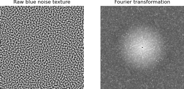
fig, axs = plt.subplots(1,5, figsize=(8,2))

for i in range(5):
    noise = blueNoise((32,32), 1.9)
    noise_rgb = np.dstack((noise,noise,noise))
    plt.imsave(f"tangle/asset/noise/blue_{ i }.png", noise_rgb)
    axs[i].imshow(noise_rgb)
    axs[i].set_axis_off()

noise_overview_path = 'tangle/tmp/noise_overview.png'
fig.savefig(noise_overview_path, bbox_inches='tight', pad_inches=0)
noise_overview_path

#pragma once
#include "assets.h"
#include "texture.h"

#include <imgui.h>
#include <imgui-SFML.h>
#include <SFML/Graphics.hpp>

In order to manage the noise texture at runtime we implement a simple NoiseSource similar to the ColorPalette class.

struct NoiseSource {
  const assets::File* current;
  sf::Texture texture;

  NoiseSource(cudaSurfaceObject_t& noise) {
    current = &assets::noise::files[0];
    texture.loadFromMemory(current->data, current->size);
    noise = bindTextureToCuda(texture);
  }

  void interact();
};

The values of the selected noise texture are also accessed similarly.

__device__ float noiseFromTexture(cudaSurfaceObject_t noisemap, int x, int y) {
  uchar4 color{};
  surf2Dread(&color, noisemap, x*sizeof(uchar4), y);
  return color.x / 255.f;
}

The interaction UI only provides a image-displaying drop down box to choose between the five different noise textures generated in this section.

void NoiseSource::interact() {
  ImGui::Image(texture, sf::Vector2f(32,20));
  ImGui::SameLine();
  if (ImGui::BeginCombo("Noise", current->name.c_str())) {
    for (unsigned i=0; i < assets::noise::file_count; ++i) {
      bool is_selected = (current == &assets::noise::files[i]);
      if (ImGui::Selectable(assets::noise::files[i].name.c_str(), is_selected)) {
        current = &assets::noise::files[i];
        texture.loadFromMemory(current->data, current->size);
        break;
      }
      if (is_selected) {
        ImGui::SetItemDefaultFocus();
      }
    }
    ImGui::EndCombo();
  }
}

We can apply a basic Gauß blurring stencil as a GLSL fragment shader to smoothen out the remaining artifacts. This common filter simply sums up the neighboring pixel colors weighted by a Gaussian normal distribution.

#version 330

uniform sampler2D texture;

layout(location = 0) out vec4 color;
layout(origin_upper_left, pixel_center_integer) in vec4 gl_FragCoord;

float kernel[7] = float[]( <<gauss-blur-filter()>> );

void main() {
  vec3 blurred = vec3(0.0);

  for (int i=-3; i <= 3; ++i) {
    for (int j=-3; j <= 3; ++j) {
      blurred += kernel[3+j] * kernel[3+i] * texelFetch(texture, ivec2(gl_FragCoord.xy) + ivec2(i,j), 0).xyz;
    }
  }

  color = vec4(blurred, 1.0);
}

As the weights used by the blur stencil stay the same for every pixel we can precompute them to speed up the shader.

def pdf(x):
    return 1/sqrt(2*pi) * exp(-1/2*x**2)

print(', '.join([ str(pdf(x).evalf()) for x in range(-3,4) ]))

0.00443184841193801, 0.0539909665131881, 0.241970724519143, 0.398942280401433, 0.241970724519143, 0.0539909665131881, 0.00443184841193801

8.6.6. Camera Controller

#pragma once
#include <cuda-samples/Common/helper_math.h>
#include <glm/gtx/quaternion.hpp>
#include "SFML/Window/Event.hpp"

A convenient way of interactively controlling the view parameters of a pinhole camera is to implement a orbiting camera. This type of camera can be rotated around a central target point using the mouse.

While translation is realized easily by adding the same shift vector to the current camera position and target point, rotation is more complex. Quaternions are a common object for expressing rotations of 3D space in a easily combinable manner.

Given 3D vectors \(v\) are easily rotated by a quaternion \(q\) using \(v^\prime = q v \overline{q}\).

glm::vec3 apply(glm::quat q, glm::vec3 v) {
  return glm::axis(q * glm::quat(0, v) * glm::conjugate(q));
}

Interactive manipulations of the rotation around a point require accumulation of individual rotations over consecutive operations. Each single operation also results of the combination of multiple basic rotations. Our Camera class is going to accumulate all rotations in a single quaternion variable _rotation.

class Camera {
private:
glm::quat _rotation;

Using the rotation quaternion we can compute all pinhole camera parameters. As they only change when a rotation is performed we store them in a set of variables.

glm::vec3 _target;
glm::vec3 _position;
glm::vec3 _forward;
glm::vec3 _right;
glm::vec3 _up;
float _distance;

Handling user input events depends on tracking some additional state to compute the delta between current and previous mouse location as well as the currently active manipulation.

float2 _mouse;

bool _rotating;
bool _moving;

bool _restricted_x;
bool _restricted_y;

The update function projects the screen space forward, right and up vectors into world space.

void update() {
  _position = _target + apply(_rotation, glm::vec3(0, _distance, 0));
  _forward = glm::normalize(_target - _position);
  _right = apply(_rotation, glm::vec3(-1, 0, 0));
  _up = apply(_rotation, glm::cross(glm::vec3(0, 1, 0), glm::vec3(-1, 0, 0)));
}

The camera's initial view will be at a distance from a given target position.

public:
Camera(float3 target, float distance):
  _distance(distance),
  _target(target.x, target.y, target.z),
  _rotating(false),
  _moving(false),
  _restricted_x(false),
  _restricted_y(false) {
  update();
}

The event handler accepts SFML-provided input events to control rotation restrictions as well as the currently selected tool.

void handle(sf::Event& event) {
  switch (event.type) {
  case sf::Event::KeyPressed:
    if (event.key.code == sf::Keyboard::LShift && !_restricted_x && !_restricted_y) {
      _restricted_x = true;
      _restricted_y = true;
    }
    break;
  case sf::Event::KeyReleased:
    if (event.key.code == sf::Keyboard::LShift) {
      _restricted_x = false;
      _restricted_y = false;
    }
    break;
  case sf::Event::MouseButtonPressed:
    if (event.mouseButton.button == sf::Mouse::Left) {
      _rotating = true;
    } else if (event.mouseButton.button == sf::Mouse::Right) {
      _moving = true;
    }
    _mouse = make_float2(event.mouseButton.x, event.mouseButton.y);
    break;
  case sf::Event::MouseButtonReleased: {
    bool restricted = _restricted_x + _restricted_y;
    _restricted_x = restricted;
    _restricted_y = restricted;
    _rotating = false;
    _moving = false;
    break;
  }

Next we change the translation and rotation vectors to zoom when the mouse wheel is turned…

  case sf::Event::MouseWheelMoved:
    _distance -= event.mouseWheel.delta * 10;
    break;

…rotate around the current screen-relative x- and z-axis…

  case sf::Event::MouseMoved:
    float2 mouse = make_float2(event.mouseMove.x, event.mouseMove.y);
    if (_rotating) {
      float2 delta = 0.005 * (mouse - _mouse);
      if (_restricted_x && _restricted_y) {
        if (std::abs(delta.x) > std::abs(delta.y)) {
          _restricted_y = false;
        } else {
          _restricted_x = false;
        }
      }
      if (_restricted_x) { delta.y = 0; }
      if (_restricted_y) { delta.x = 0; }
      glm::quat rotation_z = glm::vec3(0,0,delta.x);
      glm::quat rotation_x = glm::vec3(delta.y,0,0);
      _rotation *= glm::cross(rotation_x, rotation_z);
    }

…or move the target point while preserving rotation.

    if (_moving) {
      float2 delta = 0.04 * (mouse - _mouse);
      _target += _right*delta.x + _up*delta.y;
    }
    _mouse = mouse;
    break;
  }
  update();
}

Finally we need to provide a set of method through which the ray marching code can access the camera parametrization.

float3 getPosition() const {
  return make_float3(_position.x, _position.y, _position.z);
}
float3 getForward() const {
  return make_float3(_forward.x, _forward.y, _forward.z);
}
float3 getRight() const {
  return make_float3(_right.x, _right.y, _right.z);
}
float3 getUp() const {
  return make_float3(_up.x, _up.y, _up.z);
}
};

8.6.7. Samplers

#pragma once
#include <LLBM/base.h>

class RenderWindow;
class VolumetricRenderConfig;

All methods for mapping interfacing lattice data and image synthesizer share the common base class Sampler. This class provides a texture buffer for storing the sampled information as well as the common interface consisting of sample, render and interact methods to be called by higher-level scaffolding.

class Sampler {
protected:
const std::string _name;

DeviceTexture<float> _sample_buffer;
cudaTextureObject_t _sample_texture;
cudaSurfaceObject_t _sample_surface;

public:
Sampler(std::string name, descriptor::CuboidD<3> cuboid):
  _name(name),
  _sample_buffer(cuboid),
  _sample_texture(_sample_buffer.getTexture()),
  _sample_surface(_sample_buffer.getSurface())
 { }

const std::string& getName() const {
  return _name;
}

virtual void sample() = 0;
virtual void render(VolumetricRenderConfig& config) = 0;
virtual void interact() = 0;

};

8.6.8. Scaffolding

#pragma once
#include <LLBM/volumetric.h>
#include "camera.h"
#include "texture.h"
#include "colormap.h"
#include "noise.h"
#include "render_window.h"
#include "../sampler/sampler.h"

Any Sampler implementations we want to provide in a given simulation are maintained in a central _sampler vector. The currently selected sampling method is designated by a pointer through which the relevant Sampler::sample, Sampler::interact and Sampler::render methods are going to be called.

class VolumetricExample : public RenderWindow {
private:
std::vector<std::unique_ptr<Sampler>> _sampler;
Sampler* _current = nullptr;

We also maintain instances of the previously defined camera controller, render configuration, color palette and a noise source for jittering the ray origins.

Camera _camera;
VolumetricRenderConfig _config;
ColorPalette _palette;
NoiseSource _noise;

int _steps_per_second = 100;
int _samples_per_second = 30;

Example cases construct their samplers using the add method.

public:
template <template<typename...> class SAMPLER, typename... ARGS>
void add(ARGS&&... args) {
  _sampler.emplace_back(new SAMPLER(std::forward<ARGS>(args)...));
  _current = _sampler.back().get();
}

At its core the VolumetricExample class offers a run method that calls the example-specific simulation code via the step callable.

template <typename TIMESTEP>
void run(TIMESTEP step) {
  sf::Clock last_sample;
  sf::Clock last_frame;
  std::size_t iStep = 0;
  volatile bool simulate = true;

Next, the method instantiates a separate thread for updating the simulation state independently of visualization. This way we can e.g. vary the simulation speed or evaluate different visualization setups for a paused state.

  sf::Thread simulation([&]() {
    while (this->isOpen()) {
      if (last_sample.getElapsedTime().asSeconds() > 1.0 / _samples_per_second) {
        _current->sample();
        cudaStreamSynchronize(cudaStreamPerThread);
        last_sample.restart();
        if (simulate) {
          for (unsigned i=0; i < (1.0 / _samples_per_second) * _steps_per_second; ++i) {
            step(iStep++);
          }
        }
      }
    }
  });
  simulation.launch();

After the simulation thread has been started we enter the main visualization loop. This loop will keep running as long as the window is opened, all the while calling the draw method at the desired frame rate.

  while (this->isOpen()) {
    this->draw(
      [&](){
        <<volumetric-example-simulation-control>>
        <<volumetric-example-render-control>>
      },
      [&](sf::Event& event) {
        <<volumetric-example-handle-events>>
      }
    );
    if (last_frame.getElapsedTime().asSeconds() > 1.0 / _samples_per_second) {
      _current->render(_config);
      cudaStreamSynchronize(cudaStreamPerThread);
      last_frame.restart();
    }
  }

  simulation.wait();
}

During event handling the sampler selection can be changed interactively.

ImGui::Begin("Simulation", 0, ImGuiWindowFlags_AlwaysAutoResize);
if (ImGui::BeginCombo("Source", _current->getName().c_str())) {
  for (auto& option : _sampler) {
    if (ImGui::Selectable(option->getName().c_str(), _current == option.get())) {
      _current = option.get();
    }
  }
  ImGui::EndCombo();
}
_current->interact();
ImGui::SliderInt("Timestep/s", &_steps_per_second, 1, 1500);
ImGui::SliderInt("Samples/s", &_samples_per_second, 1, 60);
if (simulate) {
  simulate = !ImGui::Button("Pause");
} else {
  simulate =  ImGui::Button("Continue");
}
ImGui::End();

The volumetric rendering parameters that are independent of specific sampling sources are exposed in a separate window.

ImGui::Begin("Render", 0, ImGuiWindowFlags_AlwaysAutoResize);
ImGui::SliderFloat("Brightness", &_config.brightness, 0.1f, 2.f);
ImGui::SliderFloat("Delta", &_config.delta, 0.05f, 2.f);
ImGui::SliderFloat("Transparency", &_config.transparency, 0.001f, 1.f);
_palette.interact();
if (ImGui::CollapsingHeader("Details")) {
  ImGui::Checkbox("Align slices to view", &_config.align_slices_to_view);
  ImGui::SameLine();
  ImGui::Checkbox("Jitter", &_config.apply_noise);
  ImGui::SameLine();
  ImGui::Checkbox("Blur", &_config.apply_blur);
  this->setBlur(_config.apply_blur);
  if (_config.apply_noise) {
    _noise.interact();
  }
}
ImGui::End();

Any input events that are not captured by the UI framework are passed to the camera controller.

_camera.handle(event);
_config.camera_position = _camera.getPosition();
_config.camera_forward = _camera.getForward();
_config.camera_right = _camera.getRight();
_config.camera_up = _camera.getUp();
_config.canvas_size = make_uint2(this->getRenderView().width, this->getRenderView().height);

Finally a constructor is needed to instantiate the rendering environment.

VolumetricExample(descriptor::CuboidD<3> cuboid):
  RenderWindow("LiterateLB"),
  _camera(make_float3(cuboid.nX/2,cuboid.nY/2,cuboid.nZ/2), cuboid.nX),
  _config(cuboid),
  _palette(_config.palette),
  _noise(_config.noise)
{
  _config.canvas = this->getRenderSurface();
  this->setBlur(_config.apply_blur);
}

};

8.7. Window

While we did not need to directly use e.g. OpenGL instructions to produce and display visualizations, we still need some way of interfacing with the system UI and to display the textures generated from CUDA. For convenience this is done using the SFML library.

#pragma once

#include <SFML/Graphics.hpp>
#include <SFML/Graphics/Image.hpp>

#include <imgui.h>
#include <imgui-SFML.h>

#include "texture.h"
#include "assets.h"

As all 2D and 3D example simulations render their visualizations to 2D textures and provide any interactivity via the Dear ImGui library a RenderWindow wrapper class is used to collect the common scaffolding.

class RenderWindow {
private:
sf::RenderWindow _window;

sf::Sprite          _render_sprite;
sf::Texture         _render_texture;
cudaSurfaceObject_t _render_surface;
sf::Rect<int>       _render_texture_view;

sf::Shader _blur_shader;
bool _blur = false;

sf::Clock _ui_delta_clock;

public:
RenderWindow(std::string name):
  _window(sf::VideoMode(800, 600), name) {
  _render_texture.create(sf::VideoMode::getDesktopMode().width, sf::VideoMode::getDesktopMode().height);
  _render_surface = bindTextureToCuda(_render_texture);
  _render_sprite.setTexture(_render_texture);
  _render_texture_view = sf::Rect<int>(0,0,_window.getSize().x,_window.getSize().y);
  _render_sprite.setTextureRect(_render_texture_view);
  _window.setView(sf::View(sf::Vector2f(_render_texture_view.width/2, _render_texture_view.height/2),
                           sf::Vector2f(_window.getSize().x, _window.getSize().y)));
  _window.setVerticalSyncEnabled(true);
  _blur_shader.loadFromMemory(std::string(reinterpret_cast<const char*>(assets::shader::file_blur_frag)), sf::Shader::Fragment);
  _blur_shader.setUniform("texture", sf::Shader::CurrentTexture);
  ImGui::SFML::Init(_window);
  ImGuiIO& io = ImGui::GetIO();
  io.MouseDrawCursor = true;
};

bool isOpen() const {
  return _window.isOpen();
}

void setBlur(bool state) {
  _blur = state;
}

template <typename UI, typename MOUSE>
void draw(UI ui, MOUSE mouse);

cudaSurfaceObject_t getRenderSurface() {
  return _render_surface;
}

sf::Rect<int> getRenderView() {
  return _render_texture_view;
}

};

The essential component of this class is the draw method to which we can pass two functions for rendering to the window texture on one hand and for providing any UI functionality on the other hand.

template <typename UI, typename MOUSE>
void RenderWindow::draw(UI ui, MOUSE mouse) {
  sf::Event event;
  while (_window.pollEvent(event)) {
    ImGui::SFML::ProcessEvent(event);
    if (event.type == sf::Event::Closed) {
      _window.close();
    }
    if (event.type == sf::Event::Resized) {
      _render_texture_view = sf::Rect<int>(0,0,event.size.width,event.size.height);
      _render_sprite.setTextureRect(_render_texture_view);
      sf::View view(sf::Vector2f(_render_texture_view.width/2, _render_texture_view.height/2),
                    sf::Vector2f(event.size.width, event.size.height));
      _window.setView(view);
    }
    if (!ImGui::GetIO().WantCaptureMouse) {
      mouse(event);
    }
  }

  ImGui::SFML::Update(_window, _ui_delta_clock.restart());
  ui();
  _window.clear();
  if (_blur) {
    _window.draw(_render_sprite, &_blur_shader);
  } else {
    _window.draw(_render_sprite);
  }
  ImGui::SFML::Render(_window);
  _window.display();
}

This functionality is sufficient for the 2D examples but as volumetric rendering both requires significantly more scaffolding and builds on different sampler classes section 8.6.8 builds a VolumetricExample class on top of the RenderWindow.

9. Examples

#include <LLBM/base.h>
#include <LLBM/bulk.h>
#include <LLBM/boundary.h>

#include "util/render_window.h"
#include "util/texture.h"
#include "util/colormap.h"

9.1. Lid-driven Cavity

The lid-driven cavity is a very common example in the LBM community due to its simple setup while providing quite complex dynamics and extensive reference results in literature. Its geometry consists of a plain square box with solid walls and a lid moving at a constant velocity. This lid movement then induces a characteristic vortex structure inside the box.

<<example-headers>>

#include <LLBM/kernel/collect_moments.h>
#include <LLBM/kernel/collect_velocity_norm.h>

using T = float;
using DESCRIPTOR = descriptor::D2Q9;

int main() {
if (cuda::device::count() == 0) {
  std::cerr << "No CUDA devices on this system" << std::endl;
  return -1;
}
auto current = cuda::device::current::get();

After including the relevant headers and declaring which floating point precision and descriptor type to use we are ready to set up the lattice of a \(500 \times 500\) grid.

const descriptor::Cuboid<DESCRIPTOR> cuboid(500, 500);
Lattice<DESCRIPTOR,T> lattice(cuboid);

CellMaterials<DESCRIPTOR> materials(cuboid, [&cuboid](uint2 p) -> int {
  if (p.x == 0 || p.y == 0 || p.x == cuboid.nX-1) {
    return 2; // boundary cell
  } else if (p.y == cuboid.nY-1) {
    return 3; // lid cell
  } else {
    return 1; // bulk
  }
});

auto bulk_mask = materials.mask_of_material(1);
auto wall_mask = materials.mask_of_material(2);
auto lid_mask  = materials.mask_of_material(3);

The bulk collisions are going to use a relaxation time of \(0.51\) and the lid enacts a velocity of \(0.05\) lattice units. This maximum velocity can be used to scale the velocity norm for visualization.

const float tau = 0.51;
const float u_lid = 0.05;

lattice.apply(Operator(BgkCollideO(), bulk_mask, tau),
              Operator(BounceBackO(), wall_mask),
              Operator(BounceBackMovingWallO(), lid_mask, std::min(iStep*1e-3, 1.0)*u_lid, 0.f));
lattice.stream();

Every couple of time steps we execute the CollectMomentsF functor to compute the velocity moments that are then visualized using renderSliceViewToTexture.

lattice.inspect<CollectMomentsF>(bulk_mask, moments_rho.device(), moments_u.device());
renderSliceViewToTexture<<<
  dim3(cuboid.nX / 32 + 1, cuboid.nY / 32 + 1),
  dim3(32,32)
>>>(cuboid.nX, cuboid.nY,
    slice,
    [u,u_lid] __device__ (std::size_t gid) -> float {
      return length(make_float2(u[2*gid+0], u[2*gid+1])) / u_lid;
    },
    [colormap] __device__ (float x) -> float3 {
      return colorFromTexture(colormap, clamp(x, 0.f, 1.f));
    },
    window.getRenderSurface());

RenderWindow window("LDC");
cudaSurfaceObject_t colormap;
ColorPalette palette(colormap);
auto slice = [cuboid] __device__ (int iX, int iY) -> std::size_t {
               return descriptor::gid(cuboid,iX,cuboid.nY-1-iY);
             };
DeviceBuffer<T> moments_rho(cuboid.volume);
DeviceBuffer<T> moments_u(2*cuboid.volume);
T* u = moments_u.device();
std::size_t iStep = 0;

while (window.isOpen()) {
  <<ldc-simulation-step>>
  if (iStep % 100 == 0) {
    cuda::synchronize(current);
    <<ldc-visualization-step>>
    window.draw([&]() {
      ImGui::Begin("Render");
      palette.interact();
      ImGui::End();
    }, [](sf::Event&) { });
  }
  ++iStep;
}
}

The same example can also be built in 3D and visualized using volumetric rendering.

<<example-headers>>

#include "util/volumetric_example.h"
#include "sampler/velocity_norm.h"
#include "sampler/curl_norm.h"
#include "sampler/shear_layer.h"

using T = float;
using DESCRIPTOR = descriptor::D3Q19;

int main() {
if (cuda::device::count() == 0) {
  std::cerr << "No CUDA devices on this system" << std::endl;
  return -1;
}
auto current = cuda::device::current::get();

After including the relevant headers we construct the D3Q19 lattice.

const descriptor::Cuboid<DESCRIPTOR> cuboid(100, 100, 100);
Lattice<DESCRIPTOR,T> lattice(cuboid);

Before constructing the sphere we set up a basic square pipe with separate walls, in- and outlets.

CellMaterials<DESCRIPTOR> materials(cuboid, [&cuboid](uint3 p) -> int {
  if (p.x == 0 || p.x == cuboid.nX-1 || p.y == 0 || p.y == cuboid.nY-1 || p.z == cuboid.nZ-1) {
    return 2; // boundary cell
  } else if (p.z == 0) {
    return 3; // lid cell
  } else {
    return 1; // bulk
  }
});

At this point we are ready to generate masks for operator application.

auto bulk_mask = materials.mask_of_material(1);
auto wall_mask = materials.mask_of_material(2);
auto lid_mask  = materials.mask_of_material(3);

cuda::synchronize(current);

In order to model the flow we employ standard BGK collisions in the bulk. The side and bottom walls are modelled using bounce back while the lid uses moving wall bounce back.

const float tau = 0.56;
const float lid = 0.10;

lattice.apply(Operator(BgkCollideO(), bulk_mask, tau),
              Operator(BounceBackO(), wall_mask),
              Operator(BounceBackMovingWallO(), lid_mask, std::min(iStep*1e-3, 1.0)*lid, 0.f, 0.f));

lattice.stream();

Finally the volumetric renderer is used to control the simulation loop and to provide velocity, curl and shear layer visualizations.

auto none = [] __device__ (float3) -> float { return 1; };
VolumetricExample renderer(cuboid);
renderer.add<CurlNormS>(lattice, bulk_mask, none);
renderer.add<ShearLayerVisibilityS>(lattice, bulk_mask, none, make_float3(0,1,0));
renderer.add<VelocityNormS>(lattice, bulk_mask, none);
renderer.run([&](std::size_t iStep) {
  <<ldc-3d-simulation-step>>
});
}

9.2. Magnus

This example simulates the flow around two cylinders, one of which is spinning and thus invoking the Magnus effect.

<<example-headers>>

#include <LLBM/kernel/collect_moments.h>
#include <LLBM/kernel/collect_velocity_norm.h>

using T = float;
using DESCRIPTOR = descriptor::D2Q9;

int main() {
if (cuda::device::count() == 0) {
  std::cerr << "No CUDA devices on this system" << std::endl;
  return -1;
}
auto current = cuda::device::current::get();

Adding another non-spinning cylinder allows for direct comparison and also produces a Kármán vortex street.

const descriptor::Cuboid<DESCRIPTOR> cuboid(1200, 500);
Lattice<DESCRIPTOR,T> lattice(cuboid);

After setting up the lattice we define the relaxation time for the BGK collisions in the bulk and the desired rotation and inflow velocities.

const float tau = 0.52;
const float u_inflow = 0.02;
const float u_rotate = 0.08;

For the geometry we first distinguish between the bulk and walls ignoring the cylinders.

CellMaterials<DESCRIPTOR> materials(cuboid, [&cuboid](uint2 p) -> int {
  if (p.x == 0) {
    return 3; // inflow
  } else if (p.x == cuboid.nX-1) {
    return 4; // outflow
  } else if (p.y == 0 || p.y == cuboid.nY-1) {
    return 2; // wall
  } else {
    return 1; // bulk
  }
});

Using free-slip conditions at the lower and upper walls requires special handling of the edge cells to prevent artifacts from forming.

materials.set(gid(cuboid, 0,0), 2);
materials.set(gid(cuboid, 0,cuboid.nY-1), 2);
materials.set(gid(cuboid, cuboid.nX-1,0), 5);
materials.set(gid(cuboid, cuboid.nX-1,cuboid.nY-1), 5);

Both cylinders are modelled using interpolated bounce back.

auto cylinder = [cuboid] __host__ __device__ (float2 p) -> float {
                  float2 q = p - make_float2(cuboid.nX/6, 3*cuboid.nY/4);
                  float2 r = p - make_float2(cuboid.nX/6, 1*cuboid.nY/4);
                  return sdf::add(sdf::sphere(q, cuboid.nY/18),
                                  sdf::sphere(r, cuboid.nY/18));
                };

materials.sdf(cylinder, 0);
SignedDistanceBoundary bouzidi(lattice, materials, cylinder, 1, 0);

The distance from the rotating cylinder's center is used to decide where to set up the moving wall boundary.

bouzidi.setVelocity([cuboid,u_rotate](float2 p) -> float2 {
  float2 q = p - make_float2(cuboid.nX/6, 3*cuboid.nY/4);
  if (length(q) < 1.1*cuboid.nY/18) {
    return u_rotate * normalize(make_float2(-q.y, q.x));
  } else {
    return make_float2(0);
  }
});

The geometry setup is concluded by generating per-material masks to be used by the collision kernel.

auto bulk_mask = materials.mask_of_material(1);
auto wall_mask = materials.mask_of_material(2);
auto inflow_mask  = materials.mask_of_material(3);
auto outflow_mask = materials.mask_of_material(4);
auto edge_mask = materials.mask_of_material(5);

cuda::synchronize(current);

During each timestep we apply all purely local collision operators in a single fused sweep of the lattice. This is followed by calling BouzidiO on the SDF-generated boundary configuration.

lattice.apply(Operator(BgkCollideO(), bulk_mask, tau),
              Operator(BounceBackFreeSlipO(), wall_mask, WallNormal<0,1>()),
              Operator(EquilibriumVelocityWallO(), inflow_mask, std::min(iStep*1e-5, 1.)*u_inflow, WallNormal<1,0>()),
              Operator(EquilibriumDensityWallO(), outflow_mask, 1., WallNormal<-1,0>()),
              Operator(BounceBackO(), edge_mask));
lattice.apply<BouzidiO>(bouzidi.getCount(), bouzidi.getConfig());
lattice.stream();

Visualization is restricted to a plain velocity norm display in this case. More involved options will be provided for later examples.

lattice.inspect<CollectMomentsF>(bulk_mask, moments_rho.device(), moments_u.device());
renderSliceViewToTexture<<<
  dim3(cuboid.nX / 32 + 1, cuboid.nY / 32 + 1),
  dim3(32,32)
>>>(cuboid.nX, cuboid.nY,
    [cuboid] __device__ (int iX, int iY) -> std::size_t {
      return descriptor::gid(cuboid,iX,cuboid.nY-1-iY);
    },
    [u,u_rotate] __device__ (std::size_t gid) -> float {
      return length(make_float2(u[2*gid+0], u[2*gid+1])) / u_rotate;
    },
    [colormap] __device__ (float x) -> float3 {
      return colorFromTexture(colormap, clamp(x, 0.f, 1.f));
    },
    window.getRenderSurface());

The render target is provided by our RenderWindow class. We also need variables for storing the colormap and buffers for storing the computed moments.

RenderWindow window("Magnus");
cudaSurfaceObject_t colormap;
ColorPalette palette(colormap);
DeviceBuffer<T> moments_rho(cuboid.volume);
DeviceBuffer<T> moments_u(2*cuboid.volume);
T* u = moments_u.device();

Finally we run the simulation as long as the window is open while periodically calling the visualization code.

std::size_t iStep = 0;
while (window.isOpen()) {
  <<magnus-simulation-step>>
  if (iStep % 200 == 0) {
    cuda::synchronize(current);
    <<magnus-visualization-step>>
    window.draw([&]() {
      ImGui::Begin("Render");
      palette.interact();
      ImGui::End();
    }, [](sf::Event&) { });
  }
  ++iStep;
}
}

Contrasting the rotating and non-rotating cylinders we can observe both the magnus effect and the formation of a Kármán vortex street.

9.3. Flow around a Sphere

This example models a channel flow around a spherical obstacle.

<<example-headers>>

#include "util/volumetric_example.h"
#include "sampler/velocity_norm.h"
#include "sampler/curl_norm.h"
#include "sampler/q_criterion.h"

using T = float;
using DESCRIPTOR = descriptor::D3Q19;

int main() {
if (cuda::device::count() == 0) {
  std::cerr << "No CUDA devices on this system" << std::endl;
  return -1;
}
auto current = cuda::device::current::get();

After including the relevant headers we construct the D3Q19 lattice.

const descriptor::Cuboid<DESCRIPTOR> cuboid(448, 64, 64);
Lattice<DESCRIPTOR,T> lattice(cuboid);

Before constructing the sphere we set up a basic square channel with free slip walls and separate in- and outlets.

CellMaterials<DESCRIPTOR> materials(cuboid, [&cuboid](uint3 p) -> int {
  if (p.z == 0 || p.z == cuboid.nZ-1) {
    return 2; // boundary cell
  } else if (p.y == 0 || p.y == cuboid.nY-1) {
    return 3; // boundary cell
  } else if (p.x == 0) {
    return 4; // inflow cell
  } else if (p.x == cuboid.nX-1) {
    return 5; // outflow cell
  } else {
    return 1; // bulk
  }
});

As the free slip bounce back condition is not well defined at the edges we use plain bounce back instead.

for (std::size_t iX=0; iX < cuboid.nX; ++iX) {
  materials.set(gid(cuboid, iX, 0,           0), 6);
  materials.set(gid(cuboid, iX, cuboid.nY-1, 0), 6);
  materials.set(gid(cuboid, iX, 0,           cuboid.nZ-1), 6);
  materials.set(gid(cuboid, iX, cuboid.nY-1, cuboid.nZ-1), 6);
}

The sphere is modelled using a signed distance function from which we generate a configuraton of the interpolated bounce back condition.

auto obstacle = [cuboid] __host__ __device__ (float3 p) -> float {
                  float3 q = p - make_float3(cuboid.nX/6, cuboid.nY/2, cuboid.nZ/2);
                  return sdf::sphere(q, cuboid.nY/T{5});
                };
materials.sdf(obstacle, 0);
SignedDistanceBoundary bouzidi(lattice, materials, obstacle, 1, 0);

At this point themasks for operator application can be generated followed by initializing the lattice data.

auto bulk_mask    = materials.mask_of_material(1);
auto wall_mask_z  = materials.mask_of_material(2);
auto wall_mask_y  = materials.mask_of_material(3);
auto inflow_mask  = materials.mask_of_material(4);
auto outflow_mask = materials.mask_of_material(5);
auto edge_mask    = materials.mask_of_material(6);

cuda::synchronize(current);

In order to model the flow we employ standard BGK collisions in the bulk. The channel walls are modelled using (free slip) bounce back and the SDF-described sphere is represented with interpolated bounce back.

const float tau = 0.51;
const float inflow = 0.05;

lattice.apply(Operator(BgkCollideO(), bulk_mask, tau),
              Operator(BounceBackFreeSlipO(), wall_mask_z, WallNormal<0,0,1>()),
              Operator(BounceBackFreeSlipO(), wall_mask_y, WallNormal<0,1,0>()),
              Operator(EquilibriumVelocityWallO(), inflow_mask, std::min(iStep*1e-4, 1.0)*inflow, WallNormal<1,0,0>()),
              Operator(EquilibriumDensityWallO(), outflow_mask, 1, WallNormal<-1,0,0>()),
              Operator(BounceBackO(), edge_mask));
lattice.apply<BouzidiO>(bouzidi.getCount(), bouzidi.getConfig());

lattice.stream();

Finally the volumetric renderer is used to control the simulation loop and to provide velocity, curl and Q criterion visualizations.

VolumetricExample renderer(cuboid);
renderer.add<QCriterionS>(lattice, bulk_mask, obstacle);
renderer.add<CurlNormS>(lattice, bulk_mask, obstacle);
renderer.add<VelocityNormS>(lattice, bulk_mask, obstacle);
renderer.run([&](std::size_t iStep) {
  <<channel-with-sphere-simulation-step>>
});
}

9.4. Taylor-Couette

A fluid confined in the gap between two rotating cylinders with sufficient angular velocity develops interesting toroidial vortices. For this example we are going to use a special shear-layer thresholding approach for highlighting those vortices.

<<example-headers>>

#include "util/volumetric_example.h"
#include "sampler/velocity_norm.h"
#include "sampler/curl_norm.h"
#include "sampler/shear_layer.h"

using T = float;
using DESCRIPTOR = descriptor::D3Q19;

int main() {
if (cuda::device::count() == 0) {
  std::cerr << "No CUDA devices on this system" << std::endl;
  return -1;
}
auto current = cuda::device::current::get();

After including the relevant headers we construct the D3Q19 lattice.

const descriptor::Cuboid<DESCRIPTOR> cuboid(500, 96, 96);
Lattice<DESCRIPTOR,T> lattice(cuboid);

The initial geometry consists only of a cube with separated left and right boundaries.

CellMaterials<DESCRIPTOR> materials(cuboid, [&cuboid](uint3 p) -> int {
  if (p.x == 0 || p.x == cuboid.nX-1) {
    return 2;
  } else {
    return 1;
  }
});

The two cylinders are modelled using a signed distance function from which we generate a configuraton of the interpolated bounce back condition.

auto inner_cylinder = [cuboid] __host__ __device__ (float3 p) -> float {
                        float3 q = p - make_float3(0, cuboid.nY/2, cuboid.nZ/2);
                        return sdf::sphere(make_float2(q.y,q.z), cuboid.nY/T{4.5});
                      };
auto geometry = [cuboid,inner_cylinder] __host__ __device__ (float3 p) -> float {
                  float3 q = p - make_float3(0, cuboid.nY/2, cuboid.nZ/2);
                  return sdf::add(-sdf::sphere(make_float2(q.y,q.z), cuboid.nY/T{2.14}), inner_cylinder(p));
                };
materials.sdf(geometry, 0);
SignedDistanceBoundary bouzidi(lattice, materials, geometry, 1, 0);

The rotation of the inner cyclinder is modelled using a velocity field from which we generate a velocity correction for the Bouzidi boundaries.

const float wall = 0.2;

bouzidi.setVelocity([cuboid,wall](float3 p) -> float3 {
  float3 q = p - make_float3(0, cuboid.nY/2, cuboid.nZ/2);
  if (length(make_float2(q.y,q.z)) < cuboid.nY/T{2.5}) {
    return wall * normalize(make_float3(0, -q.z, q.y));
  } else {
    return make_float3(0);
  }
});

At this point we are ready to generate masks for operator application and to initialize all cells with their equilibrium.

auto bulk_mask = materials.mask_of_material(1);
auto bulk_list = materials.list_of_material(1);
auto wall_mask = materials.mask_of_material(2);
auto wall_list = materials.list_of_material(2);

cuda::synchronize(current);

Due to the large quantity of inactive cells in this example we call the collision operators on lists of cells instead of masking a full sweep of the lattice.

const float tau = 0.55;

lattice.apply<BgkCollideO>(bulk_list, tau);
lattice.apply<BounceBackO>(wall_list);
lattice.apply<BouzidiO>(bouzidi.getCount(), bouzidi.getConfig());

lattice.stream();

Finally the volumetric example renderer is used to control the simulation loop and to provide velocity, curl norm and shear layer visualizations.

VolumetricExample renderer(cuboid);
renderer.add<VelocityNormS>(lattice, bulk_mask, inner_cylinder);
renderer.add<ShearLayerVisibilityS>(lattice, bulk_mask, inner_cylinder, make_float3(1,0,0));
renderer.run([&](std::size_t iStep) {
  <<taylor-couette-simulation-step>>
});
}

After compiling the tangled program and playing around with the rendering settings for the shear layer sampler, we end up with something similar to this:

9.5. Nozzle

This is the example that was used to provide the teaser video at the start of this document. It simulates the turbulent flow that develops when a channel flow is forced through a small nozzle.

<<example-headers>>

#include "util/volumetric_example.h"
#include "sampler/velocity_norm.h"
#include "sampler/curl_norm.h"
#include "sampler/q_criterion.h"

using T = float;
using DESCRIPTOR = descriptor::D3Q19;

int main() {
if (cuda::device::count() == 0) {
  std::cerr << "No CUDA devices on this system" << std::endl;
  return -1;
}
auto current = cuda::device::current::get();

After including the relevant headers we construct the D3Q19 lattice.

const descriptor::Cuboid<DESCRIPTOR> cuboid(500, 80, 80);
Lattice<DESCRIPTOR,T> lattice(cuboid);

Before constructing the nozzle geometry we set up a basic square pipe with separate walls, in- and outlets.

CellMaterials<DESCRIPTOR> materials(cuboid, [&cuboid](uint3 p) -> int {
  if (p.y == 0 || p.y == cuboid.nY-1 || p.z == 0 || p.z == cuboid.nZ-1) {
    return 2; // boundary cell
  } else if (p.x == 0) {
    return 3; // inflow cell
  } else if (p.x == cuboid.nX-1) {
    return 4; // outflow cell
  } else {
    return 1; // bulk
  }
});

The smoothly curved nozzle is modelled using a signed distance function from which we generate a configuraton of the interpolated bounce back condition.

auto obstacle = [cuboid] __host__ __device__ (float3 p) -> float {
                  float3 q = p - make_float3(cuboid.nX/24.2f, cuboid.nY/2, cuboid.nZ/2);
                  return sdf::ssub(sdf::sphere(make_float2(q.y,q.z), cuboid.nY/T{9}),
                                   sdf::box(q, make_float3(cuboid.nX/128,cuboid.nY/2,cuboid.nZ/2)),
                                   5);
                };
materials.sdf(obstacle, 0);
SignedDistanceBoundary bouzidi(lattice, materials, obstacle, 1, 0);

At this point we are ready to generate masks for operator application and to initialize all cells with their equilibrium.

auto bulk_mask     = materials.mask_of_material(1);
auto boundary_mask = materials.mask_of_material(2);
auto inflow_mask   = materials.mask_of_material(3);
auto outflow_mask  = materials.mask_of_material(4);

cuda::synchronize(current);

In order to model the turbulence we employ Smagorinsky BGK collisions in the bulk. The channel walls are modelled using bounce back and the SDF-described nozzle is represented with interpolated bounce back.

const float tau = 0.501;
const float smagorinsky = 0.1;
const float inflow = 0.0075;

lattice.apply(Operator(SmagorinskyBgkCollideO(), bulk_mask, tau, smagorinsky),
              Operator(BounceBackO(), boundary_mask),
              Operator(EquilibriumVelocityWallO(), inflow_mask, std::min(iStep*1e-4, 1.0)*inflow, WallNormal<1,0,0>()),
              Operator(EquilibriumDensityWallO(), outflow_mask, 1, WallNormal<-1,0,0>()));
lattice.apply<BouzidiO>(bouzidi.getCount(), bouzidi.getConfig());

lattice.stream();

Finally the volumetric renderer is again used to control the simulation loop and to provide various visualizations.

VolumetricExample renderer(cuboid);
renderer.add<CurlNormS>(lattice, bulk_mask, obstacle);
renderer.add<QCriterionS>(lattice, bulk_mask, obstacle);
renderer.add<VelocityNormS>(lattice, bulk_mask, obstacle);
renderer.run([&](std::size_t iStep) {
  <<nozzle-simulation-step>>
});
}

For example, this is how the velocity magnitude visualization evolves:

10. Benchmark

10.1. Performance Measurement

#pragma once
#include <chrono>

namespace timer {

The notion of performance is directly tied to measuring timespans which is why we start out by defining some helpers to store the current time and compute how many seconds have passed between now and such a stored value.

std::chrono::time_point<std::chrono::steady_clock> now() {
  return std::chrono::steady_clock::now();
}

double secondsSince(
  std::chrono::time_point<std::chrono::steady_clock>& pit) {
  return std::chrono::duration_cast<std::chrono::duration<double>>(now() - pit).count();
}

The total performance of LBM codes is commonly measured using how many million lattice cells are updated per second, denoted as MLUPs for short.

double mlups(std::size_t nCells, std::size_t nSteps, std::chrono::time_point<std::chrono::steady_clock>& start) {
  return nCells * nSteps / (secondsSince(start) * 1e6);
}

10.2. Lid-driven Cavity

#include <LLBM/base.h>

#include <LLBM/kernel/collide.h>
#include <LLBM/kernel/bounce_back.h>
#include <LLBM/kernel/bounce_back_moving_wall.h>

#include "util/timer.h"

#include <iostream>

In order to benchmark the performance limits of our LBM code this example implements a lid driven cavity without any visual output.

using T = float;
using DESCRIPTOR = descriptor::D3Q19;

As 3D simulations are generally what is of relevance for practical applications, we are using a D3Q19 lattice of single precision values.

Lattice<DESCRIPTOR,T> lattice(cuboid);

CellMaterials<DESCRIPTOR> materials(cuboid, [&cuboid](uint3 p) -> int {
  if (p.x == 0 || p.x == cuboid.nX-1 || p.y == 0 || p.y == cuboid.nY-1 || p.z == 0) {
    return 2; // boundary cell
  } else if (p.z == cuboid.nZ-1) {
    return 3; // lid cell
  } else {
    return 1; // bulk
  }
});

auto bulk_mask = materials.mask_of_material(1);
auto box_mask  = materials.mask_of_material(2);
auto lid_mask  = materials.mask_of_material(3);

cuda::synchronize(current);

The simulation step consists of BGK collisions in the bulk and bounce back boundaries at the sides.

lattice.apply(Operator(BgkCollideO(), bulk_mask, 0.56),
              Operator(BounceBackO(), box_mask),
              Operator(BounceBackMovingWallO(), lid_mask, 0.05f, 0.f, 0.f));
lattice.stream();

The simulate function accepts a the cuboid configuration together with a step count and the floating point type to be used for lattice data and computations.

void simulate(descriptor::Cuboid<DESCRIPTOR> cuboid, std::size_t nStep) {
  auto current = cuda::device::current::get();

  <<benchmark-ldc-setup-lattice>>

  for (std::size_t iStep=0; iStep < 100; ++iStep) {
    <<benchmark-ldc-simulation-step>>
  }

  cuda::synchronize(current);

  auto start = timer::now();

  for (std::size_t iStep=0; iStep < nStep; ++iStep) {
    <<benchmark-ldc-simulation-step>>
  }

  cuda::synchronize(current);

  auto mlups = timer::mlups(cuboid.volume, nStep, start);

  std::cout << sizeof(T) << ", " << cuboid.nX << ", " << nStep << ", " << mlups << std::endl;
}

In order to easily perform many benchmarks for different configurations we implement some very basic CLI parameter handling in the main function.

int main(int argc, char* argv[]) {
  if (cuda::device::count() == 0) {
    std::cerr << "No CUDA devices on this system" << std::endl;
    return -1;
  }
  if (argc != 3) {
    std::cerr << "Invalid parameter count" << std::endl;
    return -1;
  }

  const std::size_t n     = atoi(argv[1]);
  const std::size_t steps = atoi(argv[2]);

  simulate({ n, n, n}, steps);

  return 0;
}

So once this is tangled and compiled we are ready to perform some benchmarks:

nvidia-smi --query-gpu=name --format=csv,noheader

GeForce RTX 3070

for n in $(seq $min $step $max); do
    ./benchmark-ldc $n $nSteps
done

4	64	1000	2416.56
4	80	1000	2471.92
4	96	1000	2534.33
4	112	1000	2512.18
4	128	1000	2569.58
4	144	1000	2541.29
4	160	1000	2599.92
4	176	1000	2499.82
4	192	1000	2513.63
4	208	1000	2492.54
4	224	1000	2533.04
4	240	1000	2561.12
4	256	1000	2511.97

11. References

References

[1]: Yu, H., Girimaji, S. S., and Luo, L.-S. DNS and LES of decaying isotropic turbulence with and without frame rotation using lattice Boltzmann method. Journal of Computational Physics 209, 2 (Nov. 2005), 599--616. [ DOI ]
[2]: Bouzidi, M., Firdaouss, M., and Lallemand, P. Momentum transfer of a Boltzmann-lattice fluid with boundaries. Physics of Fluids 13, 11 (Nov. 2001), 3452--3459. [ DOI ]
[3]: Krüger, T., Kusumaatmaja, H., Kuzmin, A., Shardt, O., Silva, G., and Viggen, E. M. The Lattice Boltzmann Method: Principles and Practice. Graduate Texts in Physics. Springer International Publishing, Cham, 2017. [ DOI ]
[4]: Kummerländer, A., Dorn, M., Frank, M., and Krause, M. J. Implicit Propagation of Directly Addressed Grids in Lattice Boltzmann Methods. [ DOI ]
[5]: Barth, W., and Burns, C. Virtual Rheoscopic Fluids for Flow Visualization. IEEE Transactions on Visualization and Computer Graphics 13, 6 (Nov. 2007), 1751--1758. [ DOI ]
[6]: Ulichney, R. Void-and-cluster method for dither array generation. In Electronic Imaging (1993).

1. Introduction

1.1. Kinetic Theory

1.2. Lattice Boltzmann Method

1.3. Literate Programming

2. Lattice

2.1. D2Q9

2.2. D3Q19

3. Collision Steps

3.1. Code printing

3.1.1. Custom expression transformations

3.2. Moments

3.3. Equilibrium

3.4. BGK Collision

3.5. Smagorinsky BGK Collision

4. Boundary conditions

4.1. Bounce Back

4.2. Moving Wall Bounce Back

4.3. Free Slip Boundary

4.4. Interpolated Bounce Back

4.5. Prescribed Equilibrium

4.5.1. Velocity boundary

4.5.2. Density boundary

5. Propagation Pattern

5.1. Memory

5.2. Initialization

5.3. Access

5.4. Update

6. Geometry Modeling

6.1. Sphere tracing

6.2. Constructive solid geometry

6.2.1. Primitives

6.2.2. Operators

6.3. Boundary conditions

7. Runtime Context

7.1. Memory

7.2. Descriptor Structure

7.3. Cuboid

7.4. Lattice

7.5. Operator Application

7.6. Kernel Execution

7.7. Cell List Generation

8. Visualization

8.1. Color Palettes

8.2. Velocity Norm

8.3. Curl

8.4. Rheoscopic fluid

8.4.1. Calculate shear layer normal

8.4.2. Determine shear layer visibility

8.5. Q-Criterion

8.6. Volumetric Rendering

8.6.1. Intersection Primitives

8.6.2. Pinhole Camera

8.6.3. Image Synthesis

8.6.4. Surface Shading

8.6.5. Noise

8.6.6. Camera Controller

8.6.7. Samplers

8.6.8. Scaffolding

8.7. Window

9. Examples

9.1. Lid-driven Cavity

9.2. Magnus

9.3. Flow around a Sphere

9.4. Taylor-Couette

9.5. Nozzle

10. Benchmark

10.1. Performance Measurement

10.2. Lid-driven Cavity

11. References

References

Open tasks

TODO Add more detailed explanations

TODO Expand example documentation

TODO Add literature citations for method sections

TODO Add physical dimensionalization

TODO Improve camera controller

TODO Re-add streamline visualization example